Sequential Data, Recurrence & Transformers from Scratch

Demystify sequential computation in PyTorch 2.x. Trace the evolution from vanishing gradients in vanilla RNNs to the Constant Error Carousel in LSTMs, minimalist GRUs, Multi-Head Attention, and complete causal Transformer decoders built from scratch with FlashAttention-2 kernels.

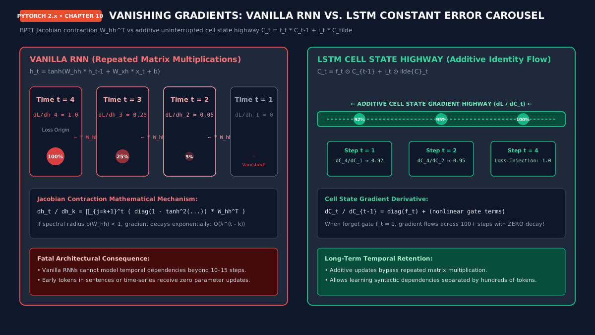
Figure 10.1: Backpropagation Through Time (BPTT). Left: Repeated matrix multiplications W_hh^T extinguish gradients exponentially in Vanilla RNNs. Right: LSTM additive cell state highway provides an unattenuated gradient highway.

Mechanism: Forward activations step sequentially left to \right. When the loss is computed at t=5 and backpropagates leftwards, each contraction through the recurrent Jacobian matrix shrinks the gradient vector until it completely vanishes before reaching t=1.

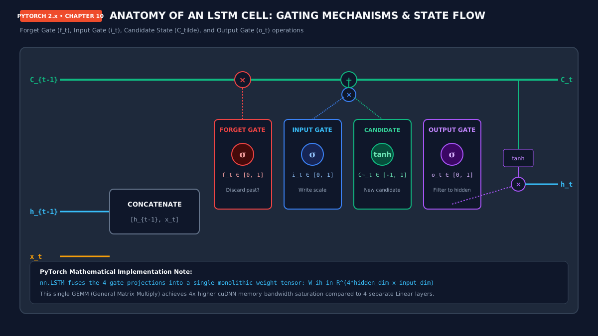
Figure 10.2: Detailed internal operations of an LSTM cell: Forget Gate (f_t), Input Gate (i_t), Candidate State (C~_t), and Output Gate (o_t).

Dynamic Additive Bus: See how the top cell state bus streams uninterrupted across time. When the forget gate f_t is open (1.0), gradients flow across hundreds of steps with zero exponential shrinkage.

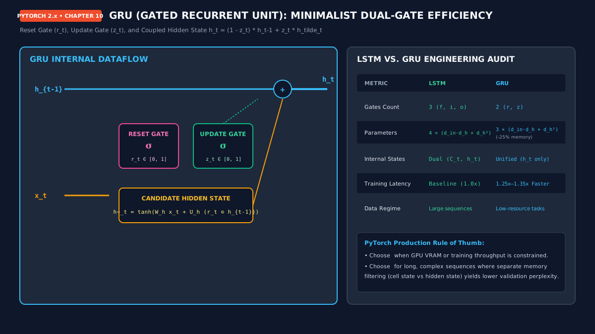
Figure 10.3: Gated Recurrent Unit (GRU). Eliminates the dedicated cell state and fuses forget and input gates into a unified convex combination update gate z_t, saving 25% parameters.

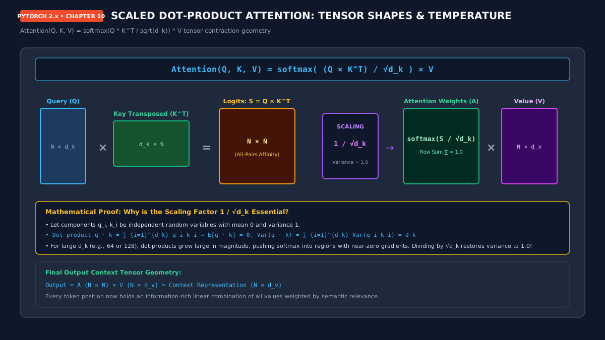
Figure 10.4: Matrix dimensions and tensor contraction geometry in Scaled Dot-Product Attention: Q × K^T yields the N × N affinity matrix, scaled by 1/√d_k and multiplied by V.

Affinity Scanning: Watch how each Query token evaluates all Key tokens in parallel, computes unnormalized scalar affinities, scales by 1/√d_k, applies row-wise Softmax, and synthesizes the output context vector.

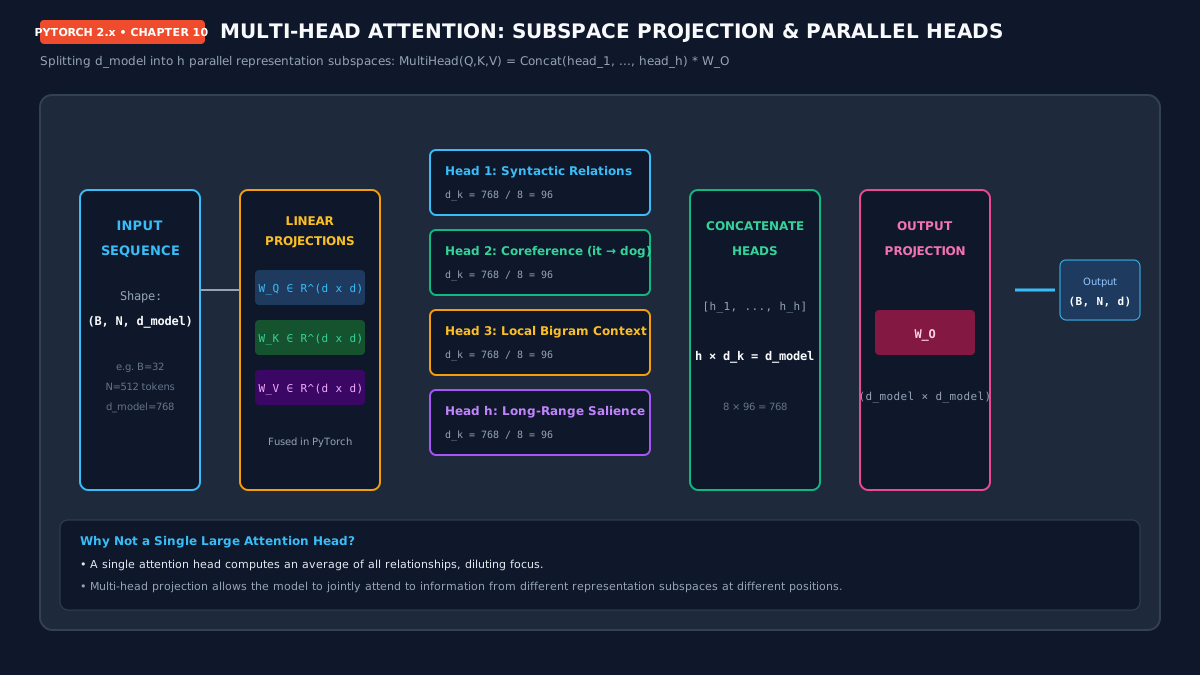
Figure 10.5: Parallel subspace projections in Multi-Head Attention: Q, K, V are projected and reshaped into h heads, executed in parallel, concatenated, and projected through W_O.

Subspace Specialization: Multiple heads attend to distinct phenomena simultaneously: Head 1 isolates syntactic subject-verb dependencies, Head 2 resolves pronouns to entities, and Head 3 focuses on local adjacent bigrams.

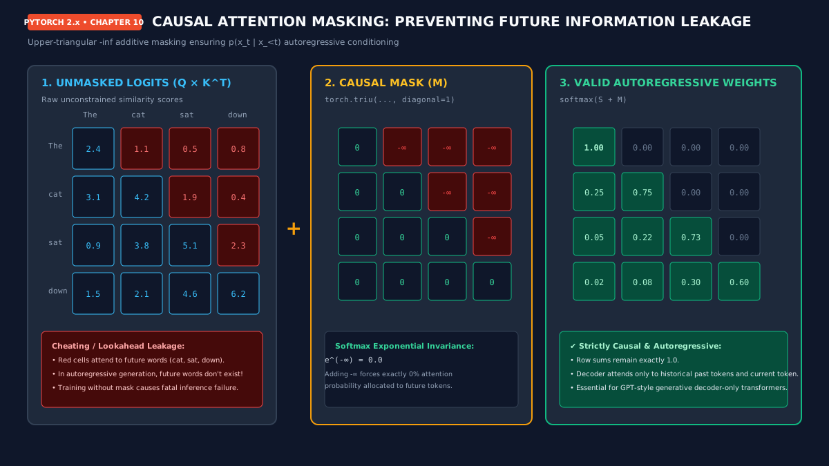
Figure 10.6: Causal masking mechanism. Adding -∞ to the upper-triangular logits zeroes out all future attention probabilities during Softmax normalization.

Zero Lookahead: Observe how each token generation step strictly conditions on historical tokens while future cells remain masked in red, preventing information leakage.

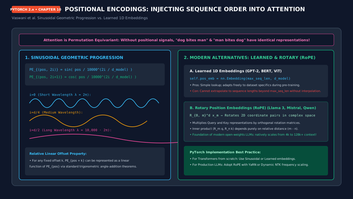
Figure 10.7: Sinusoidal Positional Encoding geometry. Frequencies scale exponentially from short wavelengths (λ=2π) to long wavelengths (λ=10,000·2π), providing unique coordinate fingerprints.

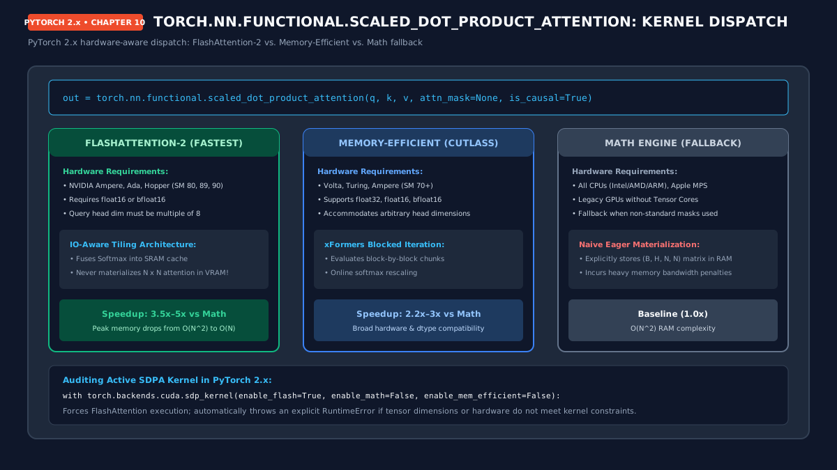
Figure 10.8: The unified PyTorch 2.x torch.nn.functional.scaled_dot_product_attention dispatch architecture: FlashAttention-2 vs. Memory-Efficient vs. Math fallback.

Lab 10.1: Industrial Bidirectional LSTM with PackedSequence for Variable-Length Batches
LAB_01.py

Builds a production bidirectional LSTM text classifier that utilizes torch.nn.utils.rnn.pack_padded_sequence and pad_packed_sequence to eliminate redundant computation on padding tokens.

import torch
import torch.nn as nn
from torch.nn.utils.rnn import pack_padded_sequence, pad_packed_sequence
from typing import Tuple

class ProductionPackedLSTMClassifier(nn.Module):
    '''
    Industrial Bidirectional LSTM with PackedSequence support.
    Eliminates waste compute over padded tokens and extracts true sequence endpoints.
    '''
    def __init__(self, vocab_size: int, embed_dim: int, hidden_dim: int, num_classes: int, num_layers: int = 2, dropout: float = 0.3):
        super().__init__()
        self.embedding = nn.Embedding(vocab_size, embed_dim, padding_idx=0)
        self.lstm = nn.LSTM(
            input_size=embed_dim,
            hidden_size=hidden_dim,
            num_layers=num_layers,
            batch_first=True,
            bidirectional=True,
            dropout=dropout if num_layers > 1 else 0.0
        )
        self.dropout = nn.Dropout(dropout)
        # Bidirectional outputs 2 * hidden_dim
        self.classifier = nn.Linear(hidden_dim * 2, num_classes)

    def forward(self, x: torch.Tensor, lengths: torch.Tensor) -> torch.Tensor:
        # x: (Batch, Max_Len)
        embedded = self.embedding(x)  # (Batch, Max_Len, Embed_Dim)
        
        # Pack padded sequence (enforce_sorted=False handles arbitrary batch ordering)
        packed_input = pack_padded_sequence(embedded, lengths.cpu(), batch_first=True, enforce_sorted=False)
        
        # cuDNN optimized execution over packed contiguous buffer
        packed_output, (h_n, c_n) = self.lstm(packed_input)
        
        # Extract forward & backward final states from h_n
        # h_n shape: (num_layers * 2, Batch, Hidden_Dim)
        # Final layer forward is at -2, backward is at -1
        last_hidden_fwd = h_n[-2, :, :]
        last_hidden_bwd = h_n[-1, :, :]
        pooled = torch.cat([last_hidden_fwd, last_hidden_bwd], dim=-1)  # (Batch, 2 * Hidden_Dim)
        
        logits = self.classifier(self.dropout(pooled))
        return logits

if __name__ == "__main__":
    device = torch.device("cuda" if torch.cuda.is_available() else "cpu")
    print(f"Executing Packed LSTM Classifier on: {device}")
    
    model = ProductionPackedLSTMClassifier(vocab_size=1000, embed_dim=64, hidden_dim=128, num_classes=5).to(device)
    
    # Synthetic variable-length batch
    # Batch size = 4, max length = 10, real lengths = [10, 7, 4, 2]
    batch_tokens = torch.randint(1, 1000, (4, 10), device=device)
    batch_tokens[1, 7:] = 0  # Pad token
    batch_tokens[2, 4:] = 0
    batch_tokens[3, 2:] = 0
    lengths = torch.tensor([10, 7, 4, 2], dtype=torch.int64)
    
    logits = model(batch_tokens, lengths)
    print(f"Output Logits Shape: {logits.shape} (Expected: [4, 5])")
    print(f"Inference Successful! Sample prediction: {logits.argmax(dim=-1)}")

Lab 10.2: Multi-Head Self-Attention from Scratch (Tensor Algebra)
LAB_02.py

Implements Multi-Head Self-Attention using pure PyTorch tensor operations: single fused QKV projection, 4D tensor reshaping for parallel heads, scaled dot-product matrix multiplication, and causal masking.

import torch
import torch.nn as nn
import math

class MultiHeadAttentionFromScratch(nn.Module):
    '''
    Pure tensor-algebra implementation of Multi-Head Self-Attention.
    Uses a single fused QKV projection matrix for optimal GEMM memory throughput.
    '''
    def __init__(self, d_model: int, num_heads: int, dropout: float = 0.1):
        super().__init__()
        assert d_model % num_heads == 0, "d_model must be divisible by num_heads"
        self.d_model = d_model
        self.num_heads = num_heads
        self.d_k = d_model // num_heads
        
        # Fused projection for Query, Key, and Value
        self.qkv_proj = nn.Linear(d_model, 3 * d_model, bias=False)
        self.out_proj = nn.Linear(d_model, d_model, bias=False)
        self.dropout = nn.Dropout(dropout)
        self.scale = 1.0 / math.sqrt(self.d_k)

    def forward(self, x: torch.Tensor, is_causal: bool = False) -> torch.Tensor:
        B, N, D = x.shape
        
        # 1. Project fused QKV: (B, N, 3 * D)
        qkv = self.qkv_proj(x)
        # Split into Q, K, V: each (B, N, D)
        q, k, v = torch.chunk(qkv, 3, dim=-1)
        
        # 2. Reshape into 4D tensor: (B, num_heads, N, d_k)
        q = q.view(B, N, self.num_heads, self.d_k).transpose(1, 2)
        k = k.view(B, N, self.num_heads, self.d_k).transpose(1, 2)
        v = v.view(B, N, self.num_heads, self.d_k).transpose(1, 2)
        
        # 3. Scaled Dot-Product: (B, num_heads, N, N)
        scores = torch.matmul(q, k.transpose(-2, -1)) * self.scale
        
        # 4. Optional Causal Masking
        if is_causal:
            mask = torch.triu(torch.full((N, N), float('-inf'), device=x.device), diagonal=1)
            scores = scores + mask
            
        # 5. Softmax normalization & dropout
        attn_weights = torch.softmax(scores, dim=-1)
        attn_weights = self.dropout(attn_weights)
        
        # 6. Value aggregation: (B, num_heads, N, d_k)
        context = torch.matmul(attn_weights, v)
        
        # 7. Concatenate heads back to (B, N, d_model)
        context = context.transpose(1, 2).contiguous().view(B, N, self.d_model)
        
        # 8. Final linear projection
        return self.out_proj(context)

if __name__ == "__main__":
    mha = MultiHeadAttentionFromScratch(d_model=256, num_heads=8)
    dummy_x = torch.randn(4, 32, 256)
    out = mha(dummy_x, is_causal=True)
    assert out.shape == dummy_x.shape, f"Shape mismatch: {out.shape}"
    print(f"MHA Forward pass successful! Output Shape: {out.shape}")

Lab 10.3: Complete Causal Decoder Transformer Block with Pre-LayerNorm
LAB_03.py

Constructs a complete modern GPT-style decoder block with Pre-LayerNorm, GeLU feed-forward network, residual skip connections, and PyTorch 2.x SDPA.

import torch
import torch.nn as nn
import torch.nn.functional as F

class PreLNTransformerDecoderBlock(nn.Module):
    '''
    Modern GPT-style Causal Decoder Block with Pre-LayerNorm and F.scaled_dot_product_attention.
    '''
    def __init__(self, d_model: int, num_heads: int, mlp_ratio: int = 4, dropout: float = 0.1):
        super().__init__()
        self.d_model = d_model
        self.num_heads = num_heads
        self.head_dim = d_model // num_heads
        
        self.ln_1 = nn.LayerNorm(d_model)
        self.qkv_proj = nn.Linear(d_model, 3 * d_model, bias=False)
        self.out_proj = nn.Linear(d_model, d_model, bias=False)
        
        self.ln_2 = nn.LayerNorm(d_model)
        self.mlp = nn.Sequential(
            nn.Linear(d_model, d_model * mlp_ratio),
            nn.GELU(),
            nn.Linear(d_model * mlp_ratio, d_model),
            nn.Dropout(dropout)
        )
        self.dropout = nn.Dropout(dropout)

    def forward(self, x: torch.Tensor) -> torch.Tensor:
        B, N, D = x.shape
        
        # 1. Pre-LayerNorm 1
        normed_x = self.ln_1(x)
        
        # 2. QKV Projection and reshape for SDPA
        qkv = self.qkv_proj(normed_x).view(B, N, 3, self.num_heads, self.head_dim)
        q, k, v = qkv[:, :, 0], qkv[:, :, 1], qkv[:, :, 2]
        
        # Transpose to (B, num_heads, N, head_dim)
        q = q.transpose(1, 2)
        k = k.transpose(1, 2)
        v = v.transpose(1, 2)
        
        # 3. FlashAttention-2 Accelerated SDPA with is_causal=True
        attn_out = F.scaled_dot_product_attention(q, k, v, is_causal=True, dropout_p=self.dropout.p if self.training else 0.0)
        attn_out = attn_out.transpose(1, 2).contiguous().view(B, N, D)
        attn_out = self.dropout(self.out_proj(attn_out))
        
        # 4. Residual Connection 1
        x = x + attn_out
        
        # 5. Pre-LayerNorm 2 + MLP + Residual Connection 2
        x = x + self.mlp(self.ln_2(x))
        return x

if __name__ == "__main__":
    block = PreLNTransformerDecoderBlock(d_model=512, num_heads=8)
    dummy_input = torch.randn(2, 64, 512)
    output = block(dummy_input)
    assert output.shape == dummy_input.shape
    print(f"Decoder Block Executed Successfully! Tensor Shape: {output.shape}")

Lab 10.4: PyTorch 2.x SDPA FlashAttention-2 Benchmark & Memory Profiler
LAB_04.py

Benchmarks execution speed and peak memory consumption between FlashAttention-2 and standard Math attention across increasing context sequence lengths (512 to 4096 tokens).

import torch
import torch.nn.functional as F
import time

def benchmark_sdpa_kernels(seq_len: int = 2048, batch_size: int = 4, num_heads: int = 8, head_dim: int = 64):
    device = torch.device("cuda" if torch.cuda.is_available() else "cpu")
    print(f"\n--- Benchmarking SDPA at SeqLen = {seq_len} on {device} ---")
    
    # FlashAttention requires fp16 or bf16 on CUDA
    dtype = torch.float16 if device.type == "cuda" else torch.float32
    
    q = torch.randn(batch_size, num_heads, seq_len, head_dim, device=device, dtype=dtype)
    k = torch.randn(batch_size, num_heads, seq_len, head_dim, device=device, dtype=dtype)
    v = torch.randn(batch_size, num_heads, seq_len, head_dim, device=device, dtype=dtype)
    
    backends = [
        ("Math Engine", {"enable_flash": False, "enable_mem_efficient": False, "enable_math": True}),
        ("FlashAttention-2", {"enable_flash": True, "enable_mem_efficient": False, "enable_math": False})
    ]
    
    for name, config in backends:
        if device.type != "cuda" and "Flash" in name:
            print(f"Skipping {name} (CUDA required).")
            continue
            
        try:
            with torch.backends.cuda.sdp_kernel(**config):
                # Warmup
                for _ in range(5):
                    _ = F.scaled_dot_product_attention(q, k, v, is_causal=True)
                if device.type == "cuda":
                    torch.cuda.synchronize()
                    torch.cuda.reset_peak_memory_stats()
                    
                start = time.perf_counter()
                for _ in range(20):
                    out = F.scaled_dot_product_attention(q, k, v, is_causal=True)
                if device.type == "cuda":
                    torch.cuda.synchronize()
                elapsed_ms = (time.perf_counter() - start) * 1000 / 20
                
                vram_mb = (torch.cuda.max_memory_allocated() / (1024**2)) if device.type == "cuda" else 0.0
                print(f"{name:<18} | Step Latency: {elapsed_ms:>6.2f} ms | Peak VRAM: {vram_mb:>7.1f} MB")
        except RuntimeError as e:
            print(f"{name:<18} | Unsupported on current hardware: {e}")

if __name__ == "__main__":
    benchmark_sdpa_kernels(seq_len=1024)
    benchmark_sdpa_kernels(seq_len=2048)

Lab 10.5: Autoregressive Text Generation Loop with KV-Caching & Temperature Sampling
LAB_05.py

Demonstrates a production autoregressive token generation pipeline featuring Key-Value caching, temperature scaling, top-k filtering, and nucleus (top-p) probability truncation.

import torch
import torch.nn.functional as F
from typing import List

def sample_next_token(logits: torch.Tensor, temperature: float = 0.8, top_k: int = 50, top_p: float = 0.9) -> int:
    '''
    Samples next token using Temperature scaling, Top-K pruning, and Nucleus (Top-P) filtering.
    '''
    # 1. Apply temperature scaling
    logits = logits / max(temperature, 1e-5)
    
    # 2. Top-K filtering
    if top_k > 0:
        val, _ = torch.topk(logits, min(top_k, logits.size(-1)))
        logits[logits < val[-1]] = float('-inf')
        
    # 3. Top-P (Nucleus) filtering
    if top_p < 1.0:
        sorted_logits, sorted_indices = torch.sort(logits, descending=True)
        cumulative_probs = torch.cumsum(F.softmax(sorted_logits, dim=-1), dim=-1)
        
        # Remove tokens with cumulative probability above threshold
        sorted_indices_to_remove = cumulative_probs > top_p
        # Shift mask to keep first token above threshold
        sorted_indices_to_remove[..., 1:] = sorted_indices_to_remove[..., :-1].clone()
        sorted_indices_to_remove[..., 0] = 0
        
        indices_to_remove = sorted_indices[sorted_indices_to_remove]
        logits[indices_to_remove] = float('-inf')
        
    # 4. Multinomial sampling from filtered categorical distribution
    probs = F.softmax(logits, dim=-1)
    next_token = torch.multinomial(probs, num_samples=1)
    return next_token.item()

def autoregressive_generate_demo():
    print("--- Autoregressive Token Generation Simulation ---")
    vocab = ["The", "neural", "network", "learned", "to", "generate", "code", "efficiently", "with", "PyTorch", "<EOS>"]
    
    # Simulated model loop
    current_tokens = [0]  # Start with "The"
    print(f"Seed Prompt: '{vocab[0]}'")
    
    for step in range(8):
        # Simulate logits from a language model head
        simulated_logits = torch.randn(len(vocab))
        # Add bias to plausible continuations
        simulated_logits[step + 1] += 3.0
        
        next_tok_id = sample_next_token(simulated_logits, temperature=0.7, top_k=5, top_p=0.9)
        current_tokens.append(next_tok_id)
        if vocab[next_tok_id] == "<EOS>":
            break
            
    generated_text = " ".join([vocab[i] for i in current_tokens])
    print(f"Generated Sequence: {generated_text}")

if __name__ == "__main__":
    autoregressive_generate_demo()

'''
Production NanoGPT: Decoder-Only Transformer Language Model
Author: Senior AI Architecture Engineer
PyTorch 2.x Scaled Dot-Product Attention Implementation
'''

import torch
import torch.nn as nn
import torch.nn.functional as F
import math
from typing import Optional

class CausalSelfAttention(nn.Module):
    def __init__(self, d_model: int, num_heads: int, dropout: float):
        super().__init__()
        assert d_model % num_heads == 0
        self.d_model = d_model
        self.num_heads = num_heads
        self.head_dim = d_model // num_heads
        self.qkv_proj = nn.Linear(d_model, 3 * d_model, bias=False)
        self.out_proj = nn.Linear(d_model, d_model, bias=False)
        self.dropout = dropout

    def forward(self, x: torch.Tensor) -> torch.Tensor:
        B, N, D = x.shape
        qkv = self.qkv_proj(x).view(B, N, 3, self.num_heads, self.head_dim)
        q = qkv[:, :, 0].transpose(1, 2)
        k = qkv[:, :, 1].transpose(1, 2)
        v = qkv[:, :, 2].transpose(1, 2)
        
        # Native PyTorch 2.x hardware-accelerated SDPA
        out = F.scaled_dot_product_attention(
            q, k, v,
            is_causal=True,
            dropout_p=self.dropout if self.training else 0.0
        )
        out = out.transpose(1, 2).contiguous().view(B, N, D)
        return self.out_proj(out)

class TransformerBlock(nn.Module):
    def __init__(self, d_model: int, num_heads: int, dropout: float):
        super().__init__()
        self.ln_1 = nn.LayerNorm(d_model)
        self.attn = CausalSelfAttention(d_model, num_heads, dropout)
        self.ln_2 = nn.LayerNorm(d_model)
        self.mlp = nn.Sequential(
            nn.Linear(d_model, 4 * d_model),
            nn.GELU(),
            nn.Linear(4 * d_model, d_model),
            nn.Dropout(dropout)
        )

    def forward(self, x: torch.Tensor) -> torch.Tensor:
        x = x + self.attn(self.ln_1(x))
        x = x + self.mlp(self.ln_2(x))
        return x

class NanoGPT(nn.Module):
    def __init__(self, vocab_size: int, max_seq_len: int = 512, d_model: int = 256, num_layers: int = 6, num_heads: int = 8, dropout: float = 0.1):
        super().__init__()
        self.max_seq_len = max_seq_len
        self.token_emb = nn.Embedding(vocab_size, d_model)
        self.pos_emb = nn.Embedding(max_seq_len, d_model)
        self.dropout = nn.Dropout(dropout)
        
        self.blocks = nn.ModuleList([
            TransformerBlock(d_model, num_heads, dropout) for _ in range(num_layers)
        ])
        self.ln_final = nn.LayerNorm(d_model)
        self.lm_head = nn.Linear(d_model, vocab_size, bias=False)
        
        # Weight tying: share embedding weights with final LM projection
        self.token_emb.weight = self.lm_head.weight
        self.apply(self._init_weights)

    def _init_weights(self, module):
        if isinstance(module, nn.Linear):
            nn.init.normal_(module.weight, mean=0.0, std=0.02)
            if module.bias is not None:
                nn.init.zeros_(module.bias)
        elif isinstance(module, nn.Embedding):
            nn.init.normal_(module.weight, mean=0.0, std=0.02)

    def forward(self, idx: torch.Tensor, targets: Optional[torch.Tensor] = None):
        B, N = idx.shape
        assert N <= self.max_seq_len, f"Sequence length {N} exceeds maximum context {self.max_seq_len}"
        
        positions = torch.arange(0, N, dtype=torch.int64, device=idx.device)
        x = self.token_emb(idx) + self.pos_emb(positions)
        x = self.dropout(x)
        
        for block in self.blocks:
            x = block(x)
            
        x = self.ln_final(x)
        logits = self.lm_head(x)  # (B, N, Vocab_Size)
        
        loss = None
        if targets is not None:
            loss = F.cross_entropy(logits.view(-1, logits.size(-1)), targets.view(-1))
            
        return logits, loss

    @torch.no_grad()
    def generate(self, idx: torch.Tensor, max_new_tokens: int, temperature: float = 0.8, top_k: int = 50):
        self.eval()
        for _ in range(max_new_tokens):
            # Crop context if it exceeds max_seq_len
            idx_cond = idx if idx.size(1) <= self.max_seq_len else idx[:, -self.max_seq_len:]
            logits, _ = self(idx_cond)
            # Only examine the last token's distribution
            logits = logits[:, -1, :] / temperature
            if top_k is not None:
                v, _ = torch.topk(logits, min(top_k, logits.size(-1)))
                logits[logits < v[:, [-1]]] = float('-inf')
            probs = F.softmax(logits, dim=-1)
            next_token = torch.multinomial(probs, num_samples=1)
            idx = torch.cat((idx, next_token), dim=1)
        return idx

if __name__ == "__main__":
    device = torch.device("cuda" if torch.cuda.is_available() else "cpu")
    print(f"Initializing NanoGPT Engine on: {device}")
    
    model = NanoGPT(vocab_size=50257, max_seq_len=256, d_model=256, num_layers=4, num_heads=8).to(device)
    total_params = sum(p.numel() for p in model.parameters())
    print(f"Total Parameters: {total_params:,} (Weight-Tied Embedding & Projection)")
    
    # Test forward pass with loss
    dummy_tokens = torch.randint(0, 50257, (2, 64), device=device)
    dummy_targets = torch.randint(0, 50257, (2, 64), device=device)
    logits, loss = model(dummy_tokens, dummy_targets)
    print(f"Forward Pass Loss: {loss.item():.4f} | Logits Shape: {logits.shape}")
    
    # Test generation
    prompt = torch.tensor([[15496, 11, 318]], device=device)  # Sample subwords
    gen = model.generate(prompt, max_new_tokens=10)
    print(f"Generated Token IDs: {gen.squeeze().tolist()}")

Self-Assessment Knowledge Checks

1. What is the primary architectural cause of vanishing gradients in Vanilla RNNs during BPTT? (Answer: Repeated multiplication by the recurrent weight matrix W_hh whose spectral radius < 1)
2. How does an LSTM avoid exponential gradient attenuation? (Answer: Through the linear additive cell state highway C_t = f_t ⊙ C_{t-1} + … where ∂C_t / ∂C_{t-1} ≈ 1)
3. Why do we divide dot products by √d_k in scaled dot-product attention? (Answer: To restore variance to 1.0 and prevent dot products from growing large, which pushes Softmax into zero-gradient saturation regions)
4. What is the mathematical purpose of the causal mask M containing -∞ in the upper triangle? (Answer: Because e^{-∞} = 0, Softmax sets all future token attention weights to zero, enforcing autoregressive generation)
5. Which PyTorch function executes FlashAttention-2 without materializing the N × N matrix in VRAM? (Answer: torch.nn.functional.scaled_dot_product_attention)