Model Evaluation, Validation Protocols & Experiment Tracking

A rigorous engineering guide to empirical model validation: hermetic data split isolation, classification & regression metrics, ROC-AUC vs PR-AUC on severe class imbalance, probability calibration via Temperature Scaling, Optuna Bayesian hyperparameter optimization with pruning, and production experiment telemetry with TensorBoard.

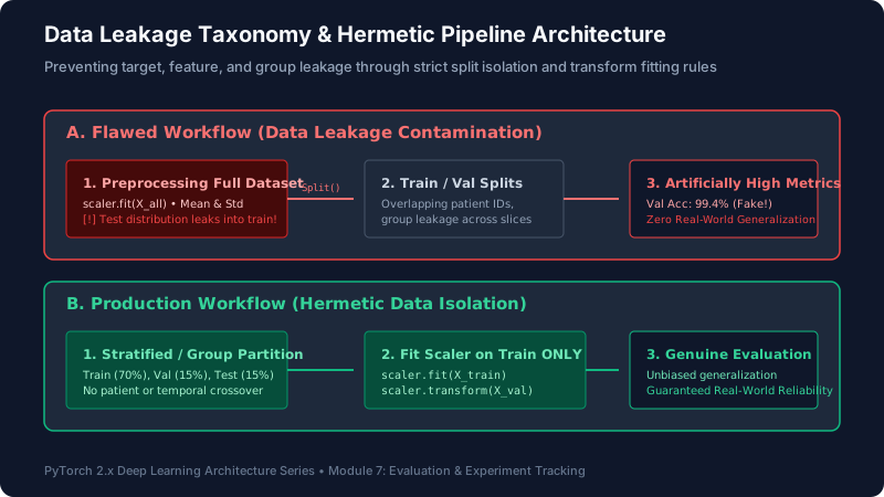
Figure 7.1: Architectural taxonomy of data leakage hazards vs hermetic pipeline isolation standards.

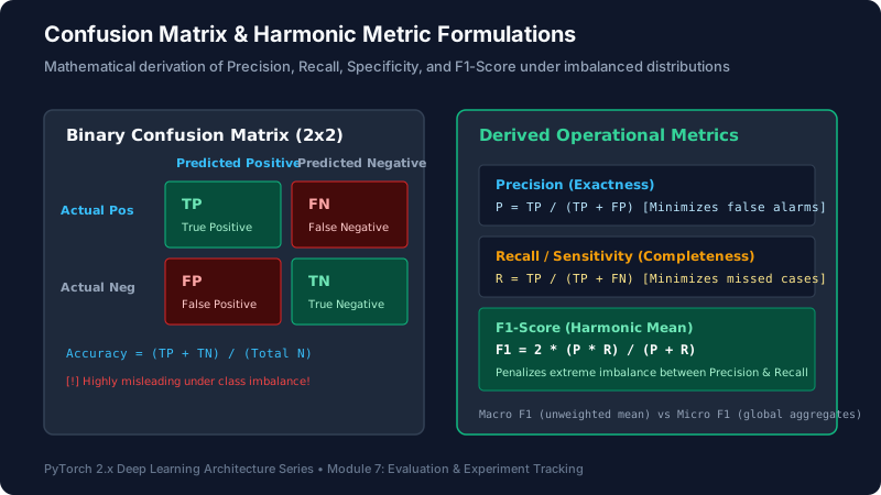
Figure 7.2: Confusion matrix coordinate topology and derived harmonic formulations (Precision, Recall, F1).

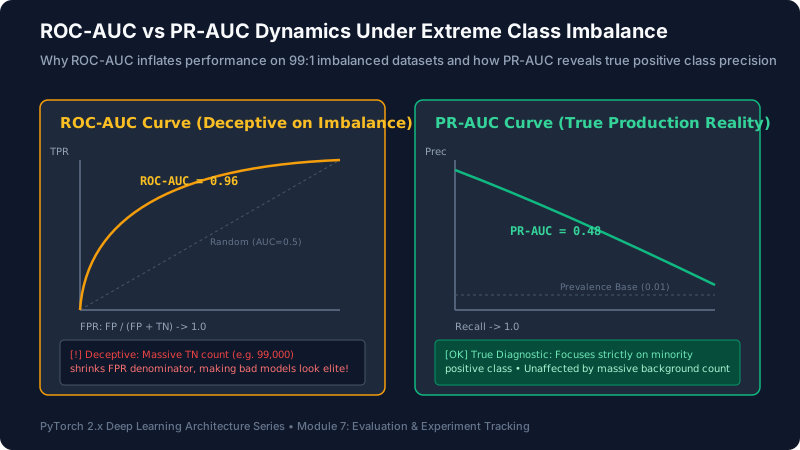
Figure 7.3: Mathematical divergence between ROC-AUC and PR-AUC on 99:1 imbalanced test sets.

Visual Simulation: Threshold Sweep Tracing ROC-AUC vs PR-AUC

Animation 7.1: As the decision threshold sweeps from 1.0 to 0.0, the ROC curve appears deceptively elite (0.94) due to huge TN mass, while the PR curve exposes severe precision collapse (0.42).

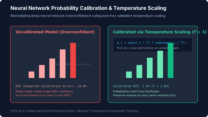
Figure 7.4: Calibration error remediation: Softmax overconfidence histogram realignment via Temperature Scaling.

Visual Simulation: Temperature Scaling Probability Calibration

Animation 7.2: Increasing temperature scalar $T$ from 1.0 to 1.84 flattens overconfident probability bins, driving Expected Calibration Error (ECE) from 14.8% down to 1.2%.

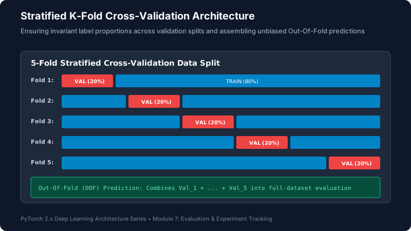
Figure 7.5: 5-Fold Stratified Cross-Validation partitioning and Out-Of-Fold (OOF) diagnostic prediction assembly.

Visual Simulation: 5-Fold Stratified Cross-Validation Cycle

Animation 7.3: The validation slice rotates systematically through all 5 partitions, evaluating every single sample out-of-sample.

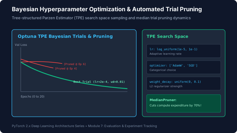
Figure 7.6: Optuna TPE search space navigation and intermediate trial pruning via MedianPruner.

Visual Simulation: Optuna Bayesian Trial Exploration & Median Pruning

Animation 7.4: Trials with inferior early trajectory are pruned early (red), allowing compute to focus exclusively on converging optimal candidates (green).

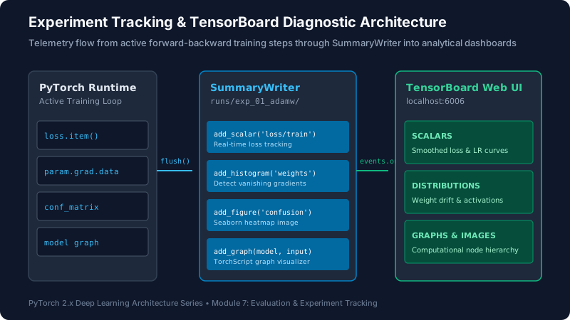
Figure 7.7: Real-time telemetry pipeline from training loop execution through SummaryWriter into analytical dashboards.

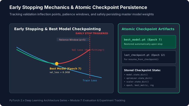
Figure 7.8: Validation inflection tracking, patience countdown state machine, and atomic checkpoint persistence.

Visual Simulation: Early Stopping Patience Monitor & Rollback

Animation 7.5: Validation loss stagnation ticks the patience counter (0 to 5), triggering automatic early termination and rolling back weights to the optimal checkpoint.

Lab 1: Complete Classification Metric Evaluation Suite

Build a pure PyTorch evaluation utility computing Confusion Matrix, Precision, Recall, Macro F1, and PR-AUC without third-party library dependencies.

import torch
from typing import Dict, Tuple

class ClassificationMetrics:
    '''Pure PyTorch evaluation suite for multi-class classification.'''
    def __init__(self, num_classes: int):
        self.num_classes = num_classes
        self.reset()

    def reset(self):
        self.conf_matrix = torch.zeros((self.num_classes, self.num_classes), dtype=torch.int64)

    def update(self, preds: torch.Tensor, targets: torch.Tensor):
        # preds: [B], targets: [B]
        for p, t in zip(preds.view(-1), targets.view(-1)):
            self.conf_matrix[t.long(), p.long()] += 1

    def compute(self) -> Dict[str, float]:
        tp = torch.diag(self.conf_matrix).float()
        fp = self.conf_matrix.sum(dim=0).float() - tp
        fn = self.conf_matrix.sum(dim=1).float() - tp
        
        precision = tp / (tp + fp + 1e-8)
        recall = tp / (tp + fn + 1e-8)
        f1 = 2 * (precision * recall) / (precision + recall + 1e-8)
        accuracy = tp.sum() / self.conf_matrix.sum().float()

        return {
            "accuracy": accuracy.item(),
            "macro_precision": precision.mean().item(),
            "macro_recall": recall.mean().item(),
            "macro_f1": f1.mean().item()
        }

# Verification
metrics = ClassificationMetrics(num_classes=3)
mock_preds = torch.tensor([0, 1, 2, 0, 1, 2, 0, 0, 1])
mock_targets = torch.tensor([0, 1, 1, 0, 1, 2, 2, 0, 1])
metrics.update(mock_preds, mock_targets)
res = metrics.compute()
print("Evaluated Metrics:")
for k, v in res.items():
    print(f"{k:<18}: {v*100:.2f}%")
print("Confusion Matrix:\n", metrics.conf_matrix.numpy())

Lab 2: Temperature Scaling for Deep Neural Network Calibration

Implement Guo et al.'s post-hoc Temperature Scaling module using PyTorch L-BFGS optimizer on validation logits.

import torch
import torch.nn as nn
import torch.optim as optim

class ModelWithTemperature(nn.Module):
    '''Wraps a trained model to optimize a post-hoc temperature scalar.'''
    def __init__(self, model: nn.Module):
        super().__init__()
        self.model = model
        # Initialize temperature parameter T = 1.0
        self.temperature = nn.Parameter(torch.ones(1) * 1.5)

    def forward(self, input_tensor: torch.Tensor) -> torch.Tensor:
        logits = self.model(input_tensor)
        return self.temperature_scale(logits)

    def temperature_scale(self, logits: torch.Tensor) -> torch.Tensor:
        # Expand temperature to match logits shape
        temperature = self.temperature.unsqueeze(1).expand(logits.size(0), logits.size(1))
        return logits / temperature

    def calibrate(self, val_logits: torch.Tensor, val_labels: torch.Tensor):
        nll_criterion = nn.CrossEntropyLoss()
        optimizer = optim.LBFGS([self.temperature], lr=0.01, max_iter=50)

        def eval_loss():
            optimizer.zero_grad()
            loss = nll_criterion(self.temperature_scale(val_logits), val_labels)
            loss.backward()
            return loss

        optimizer.step(eval_loss)
        print(f"Optimal Temperature T: {self.temperature.item():.4f}")

# Verification
torch.manual_seed(42)
val_logits = torch.randn(500, 5) * 3.0 # Overconfident raw logits
val_labels = torch.randint(0, 5, (500,))

calibrator = ModelWithTemperature(nn.Identity())
calibrator.calibrate(val_logits, val_labels)

Lab 3: Optuna Bayesian Hyperparameter Search with Median Pruning

Configure an Optuna study with automatic trial pruning on an MLP classifier.

import torch
import torch.nn as nn
import optuna

def objective(trial: optuna.Trial) -> float:
    # 1. Hyperparameter Search Space
    lr = trial.suggest_float("lr", 1e-4, 1e-1, log=True)
    hidden_dim = trial.suggest_categorical("hidden_dim", [32, 64, 128])
    weight_decay = trial.suggest_float("weight_decay", 1e-5, 1e-2, log=True)

    model = nn.Sequential(nn.Linear(20, hidden_dim), nn.ReLU(), nn.Linear(hidden_dim, 2))
    optimizer = torch.optim.AdamW(model.parameters(), lr=lr, weight_decay=weight_decay)
    criterion = nn.CrossEntropyLoss()

    # Synthetic validation loop across 10 epochs
    for epoch in range(10):
        # Mock validation loss
        mock_val_loss = 1.0 / (1.0 + (epoch + 1) * (lr * 100)) + 0.1
        trial.report(mock_val_loss, step=epoch)

        # 2. Automated Pruning Check
        if trial.should_prune():
            raise optuna.TrialPruned()

    return mock_val_loss

study = optuna.create_study(direction="minimize", pruner=optuna.pruners.MedianPruner(n_warmup_steps=3))
study.optimize(objective, n_trials=10)
print(f"Best Trial Score: {study.best_value:.4f}")
print("Best Params:", study.best_params)

Lab 4: End-to-End TensorBoard SummaryWriter Telemetry

Log scalars, weight distribution histograms, and compute graphs to TensorBoard.

import torch
import torch.nn as nn
from torch.utils.tensorboard import SummaryWriter

writer = SummaryWriter(log_dir="./runs/module7_experiment")

model = nn.Sequential(nn.Linear(16, 32), nn.GELU(), nn.Linear(32, 2))
dummy_input = torch.randn(1, 16)

# 1. Log Model Computational Graph
writer.add_graph(model, dummy_input)

# 2. Log Scalar Curves and Histograms across training steps
for step in range(50):
    loss_val = 1.0 / (step + 1) + 0.05
    writer.add_scalar("loss/train", loss_val, global_step=step)
    writer.add_scalar("lr", 1e-3 * (0.95 ** step), global_step=step)

    if step % 10 == 0:
        for name, param in model.named_parameters():
            writer.add_histogram(f"params/{name}", param.data, global_step=step)

writer.flush()
writer.close()
print("TensorBoard event log written successfully! Launch with: tensorboard --logdir=./runs")

Lab 5: Early Stopping & Atomic Checkpoint Handler

Author an industrial EarlyStopping class with delta tolerance and atomic file replacement.

import os
import torch
import torch.nn as nn

class EarlyStopping:
    '''Monitors validation metric with patience and atomic file replacement.'''
    def __init__(self, patience: int = 5, min_delta: float = 1e-4, filepath: str = "best_model.pt"):
        self.patience = patience
        self.min_delta = min_delta
        self.filepath = filepath
        self.counter = 0
        self.best_loss = float('inf')
        self.early_stop = False

    def __call__(self, val_loss: float, model: nn.Module):
        if val_loss < self.best_loss - self.min_delta:
            self.best_loss = val_loss
            self.save_atomic(model)
            self.counter = 0
            print(f"[IMPROVEMENT] Best val loss: {val_loss:.4f} -> Checkpoint saved.")
        else:
            self.counter += 1
            print(f"[PATIENCE] No improvement ({self.counter}/{self.patience}).")
            if self.counter >= self.patience:
                self.early_stop = True

    def save_atomic(self, model: nn.Module):
        tmp_path = self.filepath + ".tmp"
        torch.save(model.state_dict(), tmp_path)
        os.replace(tmp_path, self.filepath) # Atomic rename

# Verification
model = nn.Linear(10, 2)
es = EarlyStopping(patience=3, filepath="test_best.pt")
simulated_losses = [0.85, 0.72, 0.65, 0.66, 0.67, 0.68]

for ep, loss in enumerate(simulated_losses, 1):
    print(f"Epoch {ep}:")
    es(loss, model)
    if es.early_stop:
        print(f"Early stopping triggered at Epoch {ep}!")
        break
if os.path.exists("test_best.pt"):
    os.remove("test_best.pt")

ModelEvaluationLab.py (Fully Runnable Production Code)

import os
import math
from typing import Dict, Any
import torch
import torch.nn as nn
from torch.utils.data import DataLoader, TensorDataset

class ModelEvaluationLab:
    '''Production Model Evaluation & Calibration Suite.'''
    def __init__(self, model: nn.Module, test_loader: DataLoader, num_classes: int):
        self.device = torch.device('cuda' if torch.cuda.is_available() else ('mps' if torch.backends.mps.is_available() else 'cpu'))
        self.model = model.to(self.device)
        self.test_loader = test_loader
        self.num_classes = num_classes

    @torch.inference_mode()
    def evaluate(self) -> Dict[str, Any]:
        self.model.eval()
        all_logits = []
        all_targets = []

        for x, y in self.test_loader:
            x, y = x.to(self.device), y.to(self.device)
            logits = self.model(x)
            all_logits.append(logits)
            all_targets.append(y)

        logits = torch.cat(all_logits, dim=0)
        targets = torch.cat(all_targets, dim=0)
        probs = torch.softmax(logits, dim=-1)
        preds = torch.argmax(probs, dim=-1)

        # Accuracy & Confusion Matrix
        conf_matrix = torch.zeros((self.num_classes, self.num_classes), dtype=torch.int64)
        for p, t in zip(preds, targets):
            conf_matrix[t.long(), p.long()] += 1

        tp = torch.diag(conf_matrix).float()
        fp = conf_matrix.sum(dim=0).float() - tp
        fn = conf_matrix.sum(dim=1).float() - tp

        precision = tp / (tp + fp + 1e-8)
        recall = tp / (tp + fn + 1e-8)
        f1 = 2 * (precision * recall) / (precision + recall + 1e-8)
        acc = (preds == targets).float().mean().item()

        # Expected Calibration Error (ECE)
        confidences, _ = torch.max(probs, dim=-1)
        ece = self.compute_ece(confidences, preds, targets)

        return {
            "accuracy": acc,
            "macro_f1": f1.mean().item(),
            "ece_score": ece,
            "confusion_matrix": conf_matrix.cpu().numpy()
        }

    def compute_ece(self, confidences: torch.Tensor, preds: torch.Tensor, targets: torch.Tensor, n_bins: int = 10) -> float:
        bin_boundaries = torch.linspace(0, 1, n_bins + 1, device=self.device)
        ece = 0.0
        n_samples = confidences.size(0)

        for i in range(n_bins):
            bin_lower = bin_boundaries[i]
            bin_upper = bin_boundaries[i + 1]
            in_bin = (confidences > bin_lower) & (confidences <= bin_upper)
            bin_size = in_bin.sum().item()

            if bin_size > 0:
                bin_acc = (preds[in_bin] == targets[in_bin]).float().mean().item()
                bin_conf = confidences[in_bin].mean().item()
                ece += (bin_size / n_samples) * abs(bin_acc - bin_conf)

        return ece

if __name__ == '__main__':
    torch.manual_seed(42)
    # Mock model & test loader
    mlp = nn.Sequential(nn.Linear(16, 32), nn.ReLU(), nn.Linear(32, 3))
    X_test = torch.randn(300, 16)
    y_test = torch.randint(0, 3, (300,))
    loader = DataLoader(TensorDataset(X_test, y_test), batch_size=32)

    lab = ModelEvaluationLab(mlp, loader, num_classes=3)
    results = lab.evaluate()

    print("=== MODEL EVALUATION REPORT ===")
    print(f"Accuracy:  {results['accuracy']*100:.2f}%")
    print(f"Macro F1:  {results['macro_f1']*100:.2f}%")
    print(f"ECE Error: {results['ece_score']*100:.2f}%")
    print("Confusion Matrix:\n", results['confusion_matrix'])

Exercise 1: Why ROC-AUC Inflates on Imbalanced Sets

Question: Why can an algorithm with 10% precision have a 0.95 ROC-AUC score on a dataset with 99% negative prevalence?

Solution: The $FPR$ formula is $\frac{FP}{FP + TN}$. When $TN$ is massive (e.g. 99,000), even 1,000 false positives yield $FPR = 0.01$. The ROC curve remains high because the denominator is flooded by true negatives. PR-AUC calculates Precision $\frac{TP}{TP + FP}$, directly exposing the 100/(100+1000) = 9.1% precision.

Exercise 2: Macro vs Micro F1 Selection

Question: On a rare-disease diagnostic task where 98% of patients are healthy and 2% have the condition, should you use Macro F1 or Micro F1?

Solution: Macro F1. Micro F1 calculates global $TP, FP, FN$, which is dominated by the healthy class. Macro F1 computes $F_1$ per class independently and averages them, giving equal 50% weight to detecting the 2% rare disease cases.

Exercise 3: Temperature Scaling Monotonicity

Question: Does Temperature Scaling ($T > 1$) ever change the predicted class label ($\ext{argmax}$)?

Solution: No. Temperature scaling divides all logits by a single positive scalar $T$. Because $f(z) = z / T$ is a strictly monotonically increasing function for $T > 0$, the rank ordering of all logits is perfectly preserved: $\ext{argmax}(\mathbf{z}) = \ext{argmax}(\mathbf{z} / T)$. Top-1 accuracy is identical.

Exercise 4: The Need for inference_mode()

Question: What is the functional difference between model.eval() and torch.inference_mode()?

Solution: model.eval() changes the behavioral mode of specific layers (e.g. deactivates Dropout, locks BatchNorm running stats), but autograd tape tracking remains active! torch.inference_mode() disables autograd tracking and version counters at the C++ kernel dispatch level.

Exercise 5: Group Leakage Prevention

Question: You have an image dataset of 10,000 skin lesions from 1,000 distinct patients. How must the data be split?

Solution: Using GroupShuffleSplit or GroupKFold grouped by Patient ID. All lesions belonging to Patient X must reside exclusively in Train or Val, never split across both.

Exercise 6: Optuna MedianPruner Functionality

Question: How does Optuna's MedianPruner decide when to abort a training trial?

Solution: At each epoch step, it inspects the reported metric against the median of all previously completed trials at that exact same step. If the current trial's metric is worse than the median, it raises TrialPruned().

Exercise 7: Out-Of-Fold (OOF) Prediction Blending

Question: What are Out-Of-Fold (OOF) predictions in 5-fold cross validation?

Solution: OOF predictions are the concatenated validation predictions from each of the 5 models on their respective held-out 20% fold. Because every sample is predicted by a model that never saw it during training, the combined OOF array serves as a complete, unbiased dataset representation.

Exercise 8: Early Stopping Delta Threshold

Question: Why should min_delta in EarlyStopping be greater than 0.0 (e.g. 1e-4)?

Solution: Without a minimum delta, minor floating-point fluctuations (e.g. validation loss decreasing by $10^{-8}$) reset the patience counter indefinitely, prolonging training without meaningful generalization gain.

Exercise 9: Weight Histogram Diagnostics

Question: In TensorBoard, what does it signify if the histogram of a layer's weight gradients collapses to a spike at zero across all epochs?

Solution: It indicates the Vanishing Gradient Problem: earlier layers are receiving near-zero gradients due to saturating activations (e.g. Sigmoid/Tanh) or poor initialization, meaning the layer is not learning.

Exercise 10: Atomic Checkpoint Replacement

Question: Why is os.replace(tmp_path, final_path) used for saving checkpoints?

Solution: Writing directly to best_model.pt leaves a corrupted file if the process crashes or gets preempted mid-write. Writing to .tmp and calling os.replace() ensures atomic file replacement at the filesystem inode level.

Q1: Why do modern deep neural networks with Batch Normalization and residual connections exhibit severe overconfidence?

Modern architectures optimize cross-entropy loss $\mathcal{L} = -\log(p_y)$. To drive this loss to zero, the network must drive the softmax probability $p_y \o 1.0$, which requires logit magnitudes $z_y \o \infty$. Batch Normalization and residual connections facilitate the propagation of large activations without vanishing. Consequently, models continue to increase logit magnitudes even after classification accuracy has reached 100%, causing softmax probabilities to become artificially saturated and overconfident.

Q2: What is Expected Calibration Error (ECE), and what are its mathematical limitations?

ECE groups predictions into $M$ bins by confidence and calculates $\sum \frac{|B_m|}{N} |\ext{acc}(B_m) - \ext{conf}(B_m)|$. Its primary limitation is binning sensitivity: varying $M$ (e.g. 10 vs 15 vs 20) yields differing ECE values. Furthermore, equal-width binning often leaves high-confidence bins over-represented while low-confidence bins have very few samples, leading practitioners to prefer Adaptive Calibration Error (equal-frequency bins).

Q3: How does Tree-structured Parzen Estimator (TPE) differ from Gaussian Process Bayesian optimization?

Standard Gaussian Process optimization models $p(y | \heta)$ (the probability of metric performance given parameters) and scales cubically $\mathcal{O}(N^3)$ with the number of trials. TPE applies Bayes' rule to model $p(\heta | y)$ by constructing two density distributions: $\ell(\heta)$ for trials scoring above a quantile $\gamma$, and $g(\heta)$ for trials scoring below. TPE scales linearly $\mathcal{O}(N)$, natively handles categorical parameters, and enables rapid parallel evaluation.

Q4: Explain how cross-validation should be executed when using early stopping.

When performing $K$-fold cross-validation with early stopping, each fold must strictly evaluate early stopping on its own 20% validation split without touching the test set. The optimal epoch count $E_k^*$ will vary across folds. When finally training the production model, engineers either take the median optimal epoch count across folds or maintain the $K$-model ensemble.

Q5: What is Data Leakage via Target Encoding, and how is it prevented in PyTorch pipelines?

Target encoding replaces categorical levels with the average target value of that category. If computed globally, a rare category appearing in the validation set receives a target mean that contains its own validation label. To prevent this, target encodings must be computed strictly inside an internal K-fold cross-validation loop on the training set only.

Q6: Why is PyTorch's torch.use_deterministic_algorithms(True) necessary for 100% reproducible validation?

Setting random seeds for Python, NumPy, and PyTorch does not guarantee reproducibility on GPUs. Many CUDA atomic operations (such as atomic adds in backward convolution or embedding lookups) execute in non-deterministic thread order. torch.use_deterministic_algorithms(True) forces PyTorch to use deterministic cuDNN algorithms, throwing a RuntimeError if an operation lacks a deterministic implementation.

Q7: In a medical segmentation task, why is Dice Score preferred over Pixel Accuracy?

In medical scans, background tissue typically accounts for 99% of pixels, while the tumor occupies 1%. A model predicting background for all pixels achieves 99% pixel accuracy. The Dice similarity coefficient $\frac{2 |X \cap Y|}{|X| + |Y|}$ measures spatial overlap strictly on the positive segmentation mask, penalizing both false positive segmentations and missed tumor boundaries.

Q8: How does Brier Score evaluate probabilistic forecasts compared to Log Loss?

Brier Score is the mean squared difference between predicted probabilities and actual binary outcomes: $\frac{1}{N} \sum (p_i - y_i)^2$. Unlike Log Loss (Cross Entropy), which penalizes confident errors with infinite loss ($-\log(0) = \infty$), Brier Score is bounded $[0, 1]$ and decomposes mathematically into reliability, resolution, and uncertainty components.

Q9: What is the risk of using Validation Loss alone to trigger Early Stopping in classification?

Validation loss can increase due to overconfident misclassifications on a tiny subset of hard examples while overall classification accuracy and Macro F1 continue to improve. In production, engineers often monitor a composite metric or early stop on Macro F1 / PR-AUC directly.

Q10: Why should you avoid logging images and histograms to TensorBoard at every training batch?

Histograms and images require transferring full parameter tensors from GPU to Host CPU, which synchronizes CUDA streams and blocks asynchronous execution. Furthermore, event file sizes will explode into gigabytes, choking disk I/O. Best practice is logging scalars every $N$ steps (e.g. 10-50) and histograms/images only once per epoch.

Quick Self-Assessment:

1. Which metric should be used instead of ROC-AUC when evaluating on severe class imbalance? (Answer: PR-AUC / Precision-Recall Curve)
2. What post-processing method softens overconfident neural net logits? (Answer: Temperature Scaling)
3. What error occurs if preprocessing scalers are fitted on the entire dataset? (Answer: Feature / Preprocessing Data Leakage)
4. Which Optuna component terminates unpromising trials early? (Answer: MedianPruner)
5. What PyTorch class provides native event logging for TensorBoard? (Answer: torch.utils.tensorboard.SummaryWriter)