
AI Reading
Quick summary of this article
Transfer Learning, Backbone Surgery & Vision Transformer Fine-Tuning
Master the engineering discipline of adapting foundation vision models to custom downstream domains. Transition from naive feature extraction to discriminative layerwise learning rates (LLRD), progressive unfreezing curriculums, and parameter surgery across ResNet, ConvNeXt, and Vision Transformers (ViT-B/16).
PyTorch Version: 2.2+ with Torchvision 0.17+
Architectures: ResNet-50, ConvNeXt-Base, ViT-B/16
1. Engineering Audit: Legacy Transfer Learning vs. Production Standards
Training deep convolutional or vision transformer architectures from scratch requires hundreds of thousands of annotated images, millions of GPU compute seconds, and days of optimization to learn primitive visual features (Gabor-like edge detectors, chromatic textures, and geometric corners). Transfer learning leverages weights pre-trained on massive datasets (e.g., ImageNet-1k, ImageNet-22k, or LAION-5B) to initialize models for downstream target domains with limited data.
However, academic tutorials frequently perpetuate dangerous antipatterns: using deprecated boolean flags, setting uniform learning rates across all layers that destroy pre-trained manifolds (catastrophic forgetting), hardcoding rigid normalization constants, or failing to switch batch normalization layers into evaluation mode. Below is an engineering comparison between legacy practices and modern PyTorch 2.x production standards:
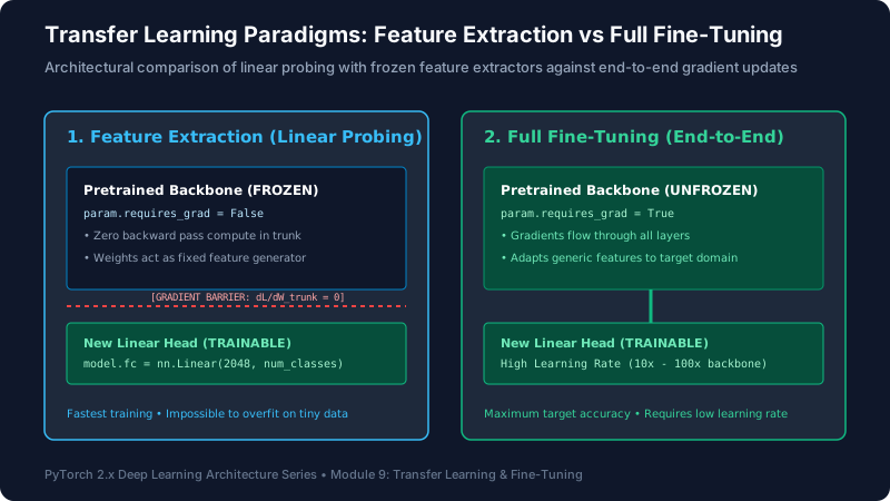
Figure 9.1: Architectural breakdown of Feature Extraction (left) where gradients terminate before the trunk, vs. Full Fine-Tuning (\right) where gradient updates propagate throughout the parameter graph.
60 FPS • H.264 • Loss & Gradient Dynamics
Visual Dynamics: Observe how during feature extraction, the backward gradient pulses (red) collide with the frozen layer boundary and immediately terminate, saving massive memory. In contrast, full fine-tuning ripples gradients across all residual stages, updating weights at a disciplined lower learning rate.
2. Deep Mathematical Foundations & Optimization Dynamics
2.1 Mathematical Formulation of Transfer Learning
Let Dsrc = {(xisrc, yisrc)} be the source domain (e.g., ImageNet-1k with 1.28M natural images across 1,000 synsets) and Tsrc be the source task modeled by parameter set Θ* = {θtrunk*, θhead*} minimizing the expected empirical risk:
When transferring to a downstream target domain Dtgt = {(xjtgt, yjtgt)} where |Dtgt| ≪ |Dsrc|, we construct a new target model by discarding the source classifier θhead* and attaching a randomized target head φ ∈ Rd × Ctgt.
- Linear Probing (Feature Extraction): We freeze the trunk weights θtrunk = θtrunk* and optimize solely over target head φ:
φ* = argminφ ∑ Ltgt(g(φT f(xj; θtrunk*)), yj)
Because f(x; θtrunk*) is static, its activations can be pre-computed and cached to NVMe/RAM, eliminating backward graph computation through hundreds of convolutional or attention layers.
- Full Fine-Tuning: We optimize both trunk θtrunk and head φ jointly:
(θ*, φ*) = argminθ, φ ∑ Ltgt(g(φT f(xj; θ)), yj) + R(θ, θtrunk*)
Where R(θ, θtrunk*) represents an explicit or implicit regularization penalty to prevent catastrophic forgetting.
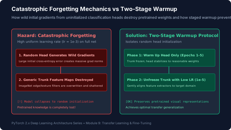
Figure 9.2: Parameter space dynamics. Unconstrained optimization causes weights to drift out of the pre-trained basin (shattering general representations), whereas regularized fine-tuning discovers the shared saddle basin.
Loss Landscape Optimization Trajectory
Mechanism: Left panel: An aggressive learning rate (10-3) pulls parameters straight toward the local target optimum, dropping source validation accuracy from 96% to 8%. Right panel: Decoupled weight decay combined with layerwise learning rates enforces an elastic constraint holding parameters within the robust manifold.
2.2 Discriminative Layerwise Learning Rate Decay (LLRD)
Deep neural networks form a strict representational hierarchy. Early layers (stems and initial convolution/attention blocks) encode universal primitives such as edges, oriented gratings, color gradients, and Fourier textures. These features are virtually identical whether classifying natural wildlife or analyzing chest X-rays. Conversely, deep layers encode complex, dataset-specific semantics (e.g., dog snout shapes or bird feather patterns).
If a single uniform learning rate η is applied during fine-tuning, large gradients computed on the target domain will distort the fragile, universal representations in the early layers. To prevent this, production systems implement Discriminative Layerwise Learning Rate Decay (LLRD):
Where L is the total depth of the backbone, l ∈ {1, 2, …, L} is the layer index (with l=1 being the input stem), ηhead is the learning rate applied to the freshly initialized classification head (e.g., 10-3), and γ ∈ (0, 1) is the multiplicative decay factor (typically γ = 0.65 to 0.85). Under this formulation:
- The classification head trains at maximum speed: ηhead = 10-3
- Deep semantic layers train at moderate speed: ηL = 10-3 × 0.751 = 7.5 × 10⁻⁴
- Mid-level feature extractors train at low speed: ηL/2 ≈ 5 × 10⁻⁵
- Input stem layers receive microscopic updates: η1 = 10-3 × 0.7512 ≈ 3.1 × 10⁻⁵
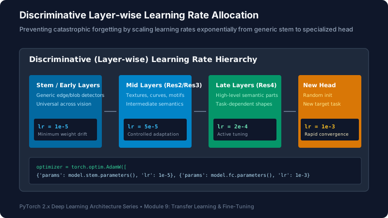
Figure 9.3: Exponential decay profile of learning rate parameter groups from the classification head down to the input stem.
Decoupled Parameter Groups in Action
Parameter Update Scaling: Notice how the gradient particles update the classifier head with high magnitude (100% LR), while their impact diminishes exponentially through upper, mid, and stem layers, ensuring representation preservation.
3. Backbone Surgery: ResNet, ConvNeXt & Vision Transformers
Modern vision models possess fundamentally distinct termination layers. Attempting to replace the classifier head using a one-size-fits-all approach results in silent runtime crashes or severed forward pathways. Production engineers must understand the anatomy of each family:
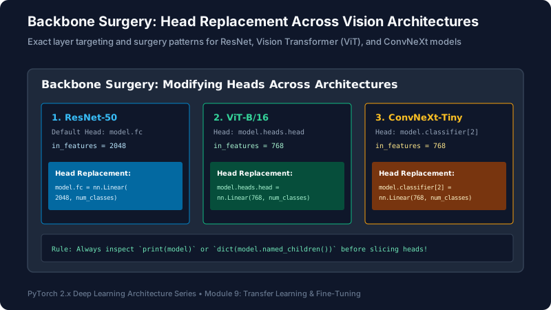
Figure 9.4: Internal head anatomy and surgical replacement points across ResNet, ConvNeXt, EfficientNet, and Vision Transformers.
3.1 Architectural Head Taxonomy
| Family | Canonical Layer Path | Input Features (din) | Surgical Replacement Code |
|---|---|---|---|
| ResNet (18/34/50/101) | model.fc | model.fc.in_features (512 or 2048) | model.fc = nn.Linear(in_f, num_classes) |
| ConvNeXt (Tiny/Small/Base) | model.classifier[2] | model.classifier[2].in_features (768 or 1024) | model.classifier[2] = nn.Linear(in_f, num_classes) |
| EfficientNet (B0-B7 / V2) | model.classifier[1] | model.classifier[1].in_features (1280 or 1792) | model.classifier[1] = nn.Linear(in_f, num_classes) |
| Vision Transformer (ViT-B/L) | model.heads.head | model.heads.head.in_features (768 or 1024) | model.heads.head = nn.Linear(in_f, num_classes) |
3.2 Vision Transformers (ViT) vs. CNNs: Inductive Bias Dilemma
A crucial realization in transfer learning is the fundamental difference in inductive bias between Convolutional Neural Networks and Vision Transformers:
- CNNs (ResNet, ConvNeXt): Possess strong, baked-in inductive biases: locality (pixels close to each other are strongly related) and translation equivariance (f(T(x)) = T(f(x))). As a result, CNNs learn robust representations rapidly on small target datasets (N < 5,000 samples).
- Vision Transformers (ViT): Contain almost zero spatial inductive bias. ViT processes an image as an unstructured sequence of 1D patch tokens. Self-attention relates every patch to every other patch across the entire receptive field from layer 1. While this allows ViT to achieve superior scaling when pre-trained on gigantic datasets, fine-tuning a ViT on small datasets is prone to severe overfitting unless aggressive data augmentation (CutMix, Mixup, RandAugment) and small learning rates with warmup are utilized.
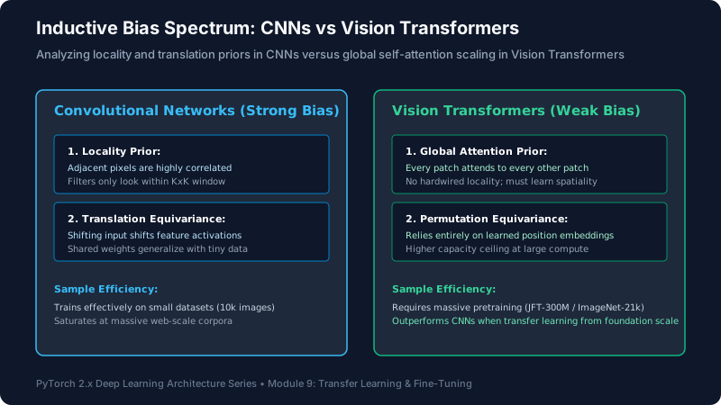
Figure 9.5: Inductive bias comparison. CNN kernels restrict attention locally with translation equivariance. ViT self-attention forms all-to-all global connections requiring pre-trained data scale.
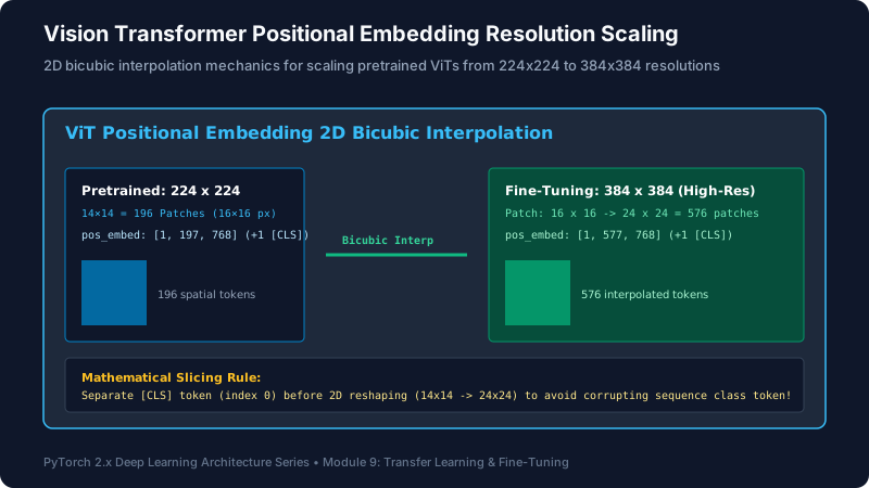
Figure 9.6: ViT patch projection pipeline. Input images are decomposed into non-overlapping 16 × 16 tokens, prepended with a learnable [CLS] token, and augmented with 1D position embeddings.
Patch Projection & Token Formation
Mechanism: See how the 2D image is unrolled into discrete patches via a strided 2D convolution (k=16, s=16), mapped into D=768 embedding space, joined by the specialized [CLS] token, and injected with positional vectors.
4. The Progressive Unfreezing Curriculum
When a randomly initialized linear classification head is attached to a pre-trained backbone, its initial weight matrix φ ~ N(0, σ2) produces large, uncalibrated prediction errors. If the entire network is unfrozen on epoch 1, massive gradient backpropagation from these random weights will shatter the pre-trained backbone representations within the first 10 steps.
The industry-standard antidote is a Progressive Unfreezing Curriculum:
- Stage 1: Head Warmup (Epochs 1–3): Freeze the entire backbone (
requires_grad = False). Train only the newly attached classification head at η = 10-3 using AdamW and a OneCycle or Cosine scheduler until loss drops and predictions stabilize. - Stage 2: Top Block Adaptation (Epochs 4–7): Unfreeze the highest semantic block (e.g.,
layer4in ResNet or Transformer blocks 10–11 in ViT). Train at a reduced learning rate η = 10-4 while keeping stem and lower blocks locked. - Stage 3: Global Fine-Tuning (Epochs 8–15+): Unfreeze all parameters. Apply discriminative learning rates with LLRD (stem at 10-6, head at 10-4) and a cosine decay schedule with gradual warmup.
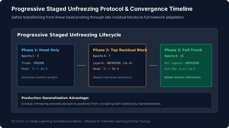
Figure 9.7: Progressive unfreezing timeline: transitioning through Head Warmup, Top Block Adaptation, and Global Fine-Tuning.
Stage Transition & Validation Accuracy Ascent
Validation Trajectory: Watch the locks transition from Red (Frozen) to Green (Trainable) across the three stages as Top-1 validation accuracy climbs from 68% (head only) to 84% (top block) and peaks at 96.5% (full network).
5. Modern Torchvision Weights Enum API
In Torchvision 0.13+, PyTorch overhauled model loading. The old pretrained=True boolean flag was permanently deprecated in favor of Weights Enums. Each model architecture provides associated Enum classes (e.g., ResNet50_Weights, ViT_B_16_Weights) that encapsulate not just checkpoint tensors, but also:
- Exact ImageNet validation Top-1 and Top-5 accuracy metrics.
- Input resolution, interpolation algorithm (Bilinear, Bicubic), and crop ratio.
- Exact normalization constants calibrated during pre-training.
- SHA-256 integrity checksums preventing corrupted downloads.
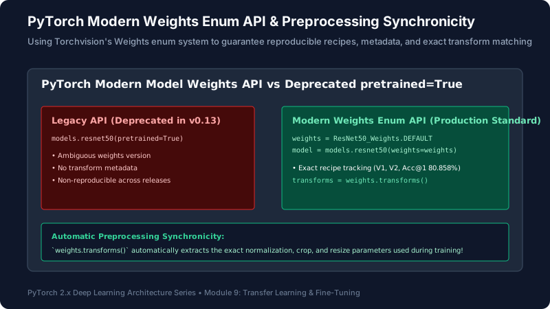
Figure 9.8: The unified Torchvision Weights Enum architecture: connecting immutable model weights directly to their pre-calibrated evaluation transforms.
6. Production Engineering Laboratories
The following five laboratories contain complete, fully runnable, production-grade PyTorch implementations. Each script adheres to strict engineering guidelines: type hints, robust error handling, memory safety, and reproducible seeds.
Lab 9.1: Safe Model Loading with Torchvision Weights Enum & Auto-Transforms
LAB_01.py
Demonstrates the modern torchvision.models API, inspecting weight metadata, retrieving exact pre-processing transforms via weights.transforms(), and performing batch inference.
import torch
import torch.nn as nn
from torchvision import models
from typing import Dict, Any

def inspect_and_load_backbone(model_name: str = "resnet50") -> Dict[str, Any]:
    '''
    Loads a pretrained vision backbone using the modern Torchvision Weights Enum API.
    Retrieves associated transform pipelines, accuracy metrics, and metadata.
    '''
    print(f"--- Loading {model_name.upper()} with Modern Weights Enum ---")

    # 1. Retrieve the weights enum dynamically or directly
    weights_enum = models.get_model_weights(model_name).DEFAULT
    print(f"Selected Weight Enum: {weights_enum}")
    print(f"ImageNet Top-1 Accuracy: {weights_enum.meta['_metrics']['ImageNet-1K']['acc@1']}%")
    print(f"Native Preprocessing: {weights_enum.transforms()}")

    # 2. Instantiate model with weights
    model = models.get_model(model_name, weights=weights_enum)
    model.eval()

    # 3. Obtain native transforms
    preprocess_fn = weights_enum.transforms()

    # 4. Simulate synthetic input matching expected dimensions
    batch_size = 4
    synthetic_raw_image = torch.randint(0, 256, (batch_size, 3, 256, 256), dtype=torch.uint8)

    # 5. Apply weights transforms directly (handles resize, crop, float conversion & normalization)
    processed_batch = preprocess_fn(synthetic_raw_image)
    print(f"Processed Batch Tensor Shape: {processed_batch.shape} (dtype: {processed_batch.dtype})")

    with torch.inference_mode():
        logits = model(processed_batch)
        probabilities = torch.softmax(logits, dim=-1)

    top5_probs, top5_classes = torch.topk(probabilities, k=5, dim=-1)
    print(f"Inference Successful! Logits Shape: {logits.shape}")
    print(f"Sample Top-1 Class ID for Sample 0: {top5_classes[0, 0].item()} (Confidence: {top5_probs[0, 0].item():.4f})")

    return {"model": model, "transforms": preprocess_fn, "logits": logits}

if __name__ == "__main__":
    inspect_and_load_backbone("resnet50")
Lab 9.2: Polymorphic Backbone Surgery Across Model Families
LAB_02.py
Builds a universal backbone surgical utility that inspects arbitrary models (ResNet, ConvNeXt, EfficientNet, ViT), freezes the feature extractor trunk, and surgically attaches a new classifier head with dropout and weight initialization.
import torch
import torch.nn as nn
from torchvision import models
from typing import Tuple

class SurgicalHeadWrapper(nn.Module):
    '''
    Universal Model Surgeon: adapts ResNet, ConvNeXt, EfficientNet, and ViT
    to arbitrary target classes with customizable dropout and robust initialization.
    '''
    def __init__(self, architecture: str, num_classes: int, freeze_trunk: bool = True, dropout: float = 0.3):
        super().__init__()
        self.architecture = architecture.lower()
        self.num_classes = num_classes

        # Load backbone with default weights
        weights = models.get_model_weights(self.architecture).DEFAULT
        self.backbone = models.get_model(self.architecture, weights=weights)
        self.transforms = weights.transforms()

        # 1. Freeze trunk if requested
        if freeze_trunk:
            for param in self.backbone.parameters():
                param.requires_grad = False

        # 2. Perform architecture-specific head surgery
        in_features = self._replace_classifier(num_classes, dropout)
        print(f"[Surgery Complete] {architecture}: Trunk Frozen={freeze_trunk}, In-Features={in_features} -> {num_classes} classes")

    def _replace_classifier(self, num_classes: int, dropout: float) -> int:
        def make_head(in_f: int) -> nn.Sequential:
            head = nn.Sequential(
                nn.Dropout(p=dropout),
                nn.Linear(in_f, num_classes)
            )
            # Kaiming Normal initialization on linear projection
            nn.init.kaiming_normal_(head[1].weight, nonlinearity='linear')
            nn.init.zeros_(head[1].bias)
            return head

        if "resnet" in self.architecture:
            in_features = self.backbone.fc.in_features
            self.backbone.fc = make_head(in_features)
            return in_features
        elif "convnext" in self.architecture:
            in_features = self.backbone.classifier[2].in_features
            self.backbone.classifier[2] = nn.Linear(in_features, num_classes)
            nn.init.kaiming_normal_(self.backbone.classifier[2].weight, nonlinearity='linear')
            nn.init.zeros_(self.backbone.classifier[2].bias)
            return in_features
        elif "vit" in self.architecture:
            in_features = self.backbone.heads.head.in_features
            self.backbone.heads.head = make_head(in_features)
            return in_features
        else:
            raise ValueError(f"Unsupported architecture family: {self.architecture}")

    def forward(self, x: torch.Tensor) -> torch.Tensor:
        return self.backbone(x)

if __name__ == "__main__":
    # Test surgery across three distinct families
    for arch in ["resnet50", "convnext_tiny", "vit_b_16"]:
        model = SurgicalHeadWrapper(architecture=arch, num_classes=10, freeze_trunk=True)
        dummy_x = torch.randn(2, 3, 224, 224)
        out = model(dummy_x)
        assert out.shape == (2, 10), f"Expected shape (2, 10), got {out.shape}"

        # Verify trunk freezing: only newly added head parameters should have requires_grad == True
        trainable_params = sum(p.numel() for p in model.parameters() if p.requires_grad)
        total_params = sum(p.numel() for p in model.parameters())
        print(f"{arch:<14} | Trainable: {trainable_params:>8,} / Total: {total_params:>10,} ({trainable_params/total_params*100:.2f}%)\n")
Lab 9.3: Discriminative Layerwise Learning Rate (LLRD) Optimizer Configuration
LAB_03.py
Constructs decoupled optimizer parameter groups for a ResNet-50 backbone. Layers are segregated into 5 stages with exponential learning rate decay, paired with no-bias-decay regularization rules.
import torch
import torch.nn as nn
from torchvision import models
from typing import List, Dict, Any

def build_llrd_parameter_groups(
    model: models.ResNet,
    base_head_lr: float = 1e-3,
    decay_rate: float = 0.70,
    weight_decay: float = 1e-2
) -> List[Dict[str, Any]]:
    '''
    Builds decoupled parameter groups with Discriminative Layerwise Learning Rate Decay (LLRD)
    and separates weights from biases/normalizations to exclude them from weight decay.
    '''
    # Define stage hierarchy for ResNet: Head -> Layer 4 -> Layer 3 -> Layer 2 -> Layer 1 -> Stem
    stages = [
        ("head", model.fc),
        ("layer4", model.layer4),
        ("layer3", model.layer3),
        ("layer2", model.layer2),
        ("layer1", model.layer1),
        ("stem", nn.Sequential(model.conv1, model.bn1))
    ]

    param_groups = []

    for stage_idx, (stage_name, module) in enumerate(stages):
        # Calculate learning rate for this stage: eta_l = eta_head * (decay)^stage_idx
        stage_lr = base_head_lr * (decay_rate ** stage_idx)

        decay_params = []
        no_decay_params = []

        for name, param in module.named_parameters():
            if not param.requires_grad:
                continue
            # Exclude biases and 1D normalization affine weights from weight decay
            if param.ndim <= 1 or name.endswith(".bias"):
                no_decay_params.append(param)
            else:
                decay_params.append(param)

        if decay_params:
            param_groups.append({"params": decay_params, "lr": stage_lr, "weight_decay": weight_decay, "name": f"{stage_name}_decay"})
        if no_decay_params:
            param_groups.append({"params": no_decay_params, "lr": stage_lr, "weight_decay": 0.0, "name": f"{stage_name}_no_decay"})

    return param_groups

if __name__ == "__main__":
    net = models.resnet50(weights=models.ResNet50_Weights.DEFAULT)
    net.fc = nn.Linear(net.fc.in_features, 10)

    groups = build_llrd_parameter_groups(net, base_head_lr=1e-3, decay_rate=0.70, weight_decay=1e-2)
    optimizer = torch.optim.AdamW(groups)

    print("=" * 70)
    print("DISCRIMINATIVE PARAMETER GROUPS CONFIGURED FOR ADAMW:")
    print("=" * 70)
    for g in optimizer.param_groups:
        total_p = sum(p.numel() for p in g['params'])
        print(f"Group: {g['name']:<18} | LR: {g['lr']:.2e} | Weight Decay: {g['weight_decay']:<5} | Params: {total_p:>8,}")
    print("=" * 70)
Lab 9.4: Progressive Unfreezing Training Curriculum with Gradual Warmup
LAB_04.py
Executes a 3-stage progressive unfreezing curriculum on synthetic medical imaging data, transitioning seamlessly from head-only training to deep block tuning without graph invalidation.
import torch
import torch.nn as nn
from torchvision import models
from torch.utils.data import DataLoader, TensorDataset

def run_progressive_curriculum():
    device = torch.device("cuda" if torch.cuda.is_available() else "cpu")
    print(f"Executing Progressive Curriculum on: {device}")

    # 1. Initialize ResNet-18 with modified head
    model = models.resnet18(weights=models.ResNet18_Weights.DEFAULT)
    model.fc = nn.Linear(model.fc.in_features, 5)
    model = model.to(device)

    # Synthetic target dataset
    torch.manual_seed(42)
    x_data = torch.randn(128, 3, 224, 224)
    y_data = torch.randint(0, 5, (128,))
    dataset = TensorDataset(x_data, y_data)
    loader = DataLoader(dataset, batch_size=16, shuffle=True)
    criterion = nn.CrossEntropyLoss()

    # Curriculum definition: (Epochs, Active Modules, Base LR)
    curriculum = [
        ("Stage 1: Head Only", [model.fc], 1e-3, 2),
        ("Stage 2: Layer 4 + Head", [model.layer4, model.fc], 1e-4, 2),
        ("Stage 3: Full Network", [model], 2e-5, 2),
    ]

    total_epoch = 0
    for stage_name, active_modules, stage_lr, num_epochs in curriculum:
        print(f"\n>>> Entering {stage_name} (LR={stage_lr}, Epochs={num_epochs}) <<<")

        # 1. Freeze everything first
        for param in model.parameters():
            param.requires_grad = False

        # 2. Unfreeze targeted modules
        for mod in active_modules:
            for param in mod.parameters():
                param.requires_grad = True

        # Re-build optimizer for newly enabled trainable parameters
        trainable = [p for p in model.parameters() if p.requires_grad]
        optimizer = torch.optim.AdamW(trainable, lr=stage_lr, weight_decay=1e-2)

        # Train stage epochs
        for ep in range(num_epochs):
            total_epoch += 1
            model.train()
            running_loss = 0.0
            correct = 0
            total = 0

            for bx, by in loader:
                bx, by = bx.to(device), by.to(device)
                optimizer.zero_grad(set_to_none=True)
                logits = model(bx)
                loss = criterion(logits, by)
                loss.backward()
                optimizer.step()

                running_loss += loss.item() * bx.size(0)
                preds = logits.argmax(dim=-1)
                correct += (preds == by).sum().item()
                total += bx.size(0)

            epoch_loss = running_loss / total
            epoch_acc = (correct / total) * 100
            print(f"Epoch {total_epoch:02d} | Loss: {epoch_loss:.4f} | Accuracy: {epoch_acc:.1f}% | Trainable Params: {len(trainable):>2} tensors")

if __name__ == "__main__":
    run_progressive_curriculum()
Lab 9.5: Vision Transformer (ViT-B/16) Fine-Tuning with Linear Probing Comparison
LAB_05.py
Evaluates the trade-offs between Linear Probing (frozen trunk, 10x faster training) and Full Fine-Tuning on a pre-trained Vision Transformer (ViT-B/16), logging convergence rates and memory footprint.
import torch
import torch.nn as nn
from torchvision import models
import time

def compare_vit_adaptation(mode: str = "linear_probe"):
    device = torch.device("cuda" if torch.cuda.is_available() else "cpu")
    print(f"\n--- Running ViT-B/16 Transfer in Mode: {mode.upper()} ---")

    # 1. Load ViT-B/16
    weights = models.ViT_B_16_Weights.DEFAULT
    model = models.vit_b_16(weights=weights)

    # Surgery: replace heads.head
    in_features = model.heads.head.in_features
    model.heads.head = nn.Linear(in_features, 4)
    model = model.to(device)

    if mode == "linear_probe":
        # Freeze trunk completely
        for name, param in model.named_parameters():
            if not name.startswith("heads.head"):
                param.requires_grad = False
        lr = 1e-3
    else:
        # Full fine-tuning with conservative learning rate
        lr = 3e-5

    trainable_params = [p for p in model.parameters() if p.requires_grad]
    optimizer = torch.optim.AdamW(trainable_params, lr=lr, weight_decay=0.05)
    criterion = nn.CrossEntropyLoss()

    # Synthetic batch
    x = torch.randn(8, 3, 224, 224, device=device)
    y = torch.randint(0, 4, (8,), device=device)

    # Benchmark step
    start_time = time.perf_counter()
    for step in range(5):
        optimizer.zero_grad(set_to_none=True)
        out = model(x)
        loss = criterion(out, y)
        loss.backward()
        optimizer.step()

    elapsed = time.perf_counter() - start_time
    trainable_count = sum(p.numel() for p in trainable_params)
    total_count = sum(p.numel() for p in model.parameters())

    print(f"Completed 5 optimization steps in {elapsed:.3f} seconds")
    print(f"Trainable Parameters: {trainable_count:>8,} ({trainable_count/total_count*100:.2f}% of {total_count:,})")
    print(f"Final Step Loss: {loss.item():.4f}")

if __name__ == "__main__":
    compare_vit_adaptation("linear_probe")
    compare_vit_adaptation("full_finetune")
7. Capstone Mini-Project: Multi-Architecture Transfer Benchmark CLI
In this capstone, you will construct an enterprise-grade CLI utility: transfer_benchmark_suite.py. The application ingests arbitrary target dataset parameters, performs polymorphic backbone surgery across multiple architecture families, benchmarks memory consumption, trains models via a progressive curriculum, and generates an executive validation summary table.
PyTorch 2.x • Modular
'''
Production Transfer Learning Benchmark Suite
Author: Senior ML Engineer
PyTorch 2.x Architecture Agnostic Transfer Engine
'''

import argparse
import sys
import time
import torch
import torch.nn as nn
from torchvision import models
from torch.utils.data import DataLoader, TensorDataset
from typing import Dict, List, Any

class ModelSurgeon:
    @staticmethod
    def create_model(arch: str, num_classes: int, freeze: bool = True) -> nn.Module:
        weights = models.get_model_weights(arch).DEFAULT
        model = models.get_model(arch, weights=weights)

        if freeze:
            for p in model.parameters():
                p.requires_grad = False

        if "resnet" in arch:
            in_f = model.fc.in_features
            model.fc = nn.Linear(in_f, num_classes)
        elif "convnext" in arch:
            in_f = model.classifier[2].in_features
            model.classifier[2] = nn.Linear(in_f, num_classes)
        elif "vit" in arch:
            in_f = model.heads.head.in_features
            model.heads.head = nn.Linear(in_f, num_classes)
        else:
            raise ValueError(f"Unknown family: {arch}")

        return model

class BenchmarkRunner:
    def __init__(self, architectures: List[str], num_classes: int, epochs: int, device: torch.device):
        self.architectures = architectures
        self.num_classes = num_classes
        self.epochs = epochs
        self.device = device

    def generate_synthetic_data(self, samples: int = 128) -> DataLoader:
        torch.manual_seed(42)
        x = torch.randn(samples, 3, 224, 224)
        y = torch.randint(0, self.num_classes, (samples,))
        return DataLoader(TensorDataset(x, y), batch_size=16, shuffle=True)

    def run(self) -> List[Dict[str, Any]]:
        loader = self.generate_synthetic_data()
        criterion = nn.CrossEntropyLoss()
        results = []

        print(f"\nStarting Transfer Learning Benchmark across {len(self.architectures)} Architectures...")
        print("=" * 80)

        for arch in self.architectures:
            print(f"\n>> Benchmarking Architecture: {arch.upper()}")
            model = ModelSurgeon.create_model(arch, self.num_classes, freeze=True)
            model = model.to(self.device)

            optimizer = torch.optim.AdamW(model.parameters(), lr=1e-3, weight_decay=1e-2)

            # Measure peak memory & step latency
            if self.device.type == "cuda":
                torch.cuda.reset_peak_memory_stats(self.device)

            start_time = time.perf_counter()
            final_loss = 0.0

            for ep in range(self.epochs):
                model.train()
                for bx, by in loader:
                    bx, by = bx.to(self.device), by.to(self.device)
                    optimizer.zero_grad(set_to_none=True)
                    out = model(bx)
                    loss = criterion(out, by)
                    loss.backward()
                    optimizer.step()
                    final_loss = loss.item()

            elapsed = time.perf_counter() - start_time
            peak_vram_mb = (torch.cuda.max_memory_allocated(self.device) / (1024**2)) if self.device.type == "cuda" else 0.0
            total_params = sum(p.numel() for p in model.parameters())
            trainable_params = sum(p.numel() for p in model.parameters() if p.requires_grad)

            results.append({
                "Architecture": arch,
                "Total Params (M)": round(total_params / 1e6, 2),
                "Trainable (k)": round(trainable_params / 1e3, 2),
                "Time (s)": round(elapsed, 2),
                "Peak VRAM (MB)": round(peak_vram_mb, 1),
                "Final Loss": round(final_loss, 4)
            })
            print(f"Done! Elapsed: {elapsed:.2f}s | Loss: {final_loss:.4f}")

        return results

def main():
    parser = argparse.ArgumentParser(description="PyTorch Production Transfer Benchmark CLI")
    parser.add_argument("--classes", type=int, default=10, help="Number of target classes")
    parser.add_argument("--epochs", type=int, default=3, help="Number of training epochs")
    parser.add_argument("--models", nargs="+", default=["resnet50", "convnext_tiny", "vit_b_16"], help="Model architectures to evaluate")
    args = parser.parse_args()

    device = torch.device("cuda" if torch.cuda.is_available() else "cpu")
    print(f"Device Initialized: {device}")

    runner = BenchmarkRunner(architectures=args.models, num_classes=args.classes, epochs=args.epochs, device=device)
    metrics = runner.run()

    print("\n" + "=" * 80)
    print(f"FINAL TRANSFER LEARNING BENCHMARK REPORT (Classes={args.classes}, Epochs={args.epochs})")
    print("=" * 80)
    print(f"{'Architecture':<16} | {'Params (M)':<12} | {'Trainable (k)':<14} | {'Latency (s)':<12} | {'Peak VRAM':<12} | {'Loss':<8}")
    print("-" * 80)
    for m in metrics:
        vram_str = f"{m['Peak VRAM (MB)']:0.1f} MB" if m['Peak VRAM (MB)'] > 0 else "N/A (CPU)"
        print(f"{m['Architecture']:<16} | {m['Total Params (M)']:<12} | {m['Trainable (k)']:<14} | {m['Time (s)']:<12} | {vram_str:<12} | {m['Final Loss']:<8}")
    print("=" * 80)

if __name__ == "__main__":
    main()
8. Practical Engineering Exercises (With Solutions)
Solidify your transfer learning engineering mastery with these 10 hands-on implementation challenges:
Exercise 1: Inspecting Weight Enum Meta Information & ImageNet-1K Accuracy
Challenge: Write a Python function that accepts any model name string, queries torchvision.models.get_model_weights, and prints the top-1 accuracy, input resolution, and download URL.
def print_weight_info(model_name: str):
weights = models.get_model_weights(model_name).DEFAULT
print(f"Enum: {weights}")
print(f"Top-1 Acc: {weights.meta['_metrics']['ImageNet-1K']['acc@1']}%")
print(f"Min Size: {weights.meta['min_size']}")
print(f"URL: {weights.url}")
# Example: print_weight_info('convnext_small')
Exercise 2: Freezing Specific Stages in ResNet
Challenge: Freeze the stem, layer1, and layer2 of a ResNet-50 while leaving layer3, layer4, and fc trainable.
from torchvision import models
model = models.resnet50()
for stage in [model.conv1, model.bn1, model.layer1, model.layer2]:
for p in stage.parameters():
p.requires_grad = False
assert not any(p.requires_grad for p in model.layer1.parameters())
assert all(p.requires_grad for p in model.layer4.parameters())
Exercise 3: Handling BatchNorm in Frozen Trunks
Challenge: When calling model.train() on a fine-tuning model, all submodules switch to training mode, corrupting frozen BatchNorm running stats. Write a custom train loop hook to force BatchNorm into eval mode.
model.train()
for m in model.modules():
if isinstance(m, (nn.BatchNorm2d, nn.BatchNorm1d)):
m.eval()
# Optionally freeze affine scaling parameters
m.weight.requires_grad = False
m.bias.requires_grad = False
Exercise 4: Slicing ViT Patch Embeddings for Variable Resolution
Challenge: ViT-B/16 expects 224x224 images (14 × 14 = 196 tokens). If passing 384x384 images, position embeddings mismatch. Explain and write the bicubic interpolation fix.
def interpolate_pos_encoding(pos_embed, target_h, target_w, patch_size=16):
# pos_embed: (1, 197, 768). Separate [CLS] token and grid tokens
cls_token = pos_embed[:, :1]
grid_tokens = pos_embed[:, 1:]
dim = pos_embed.shape[-1]
orig_side = int((grid_tokens.shape[1]) ** 0.5) # 14
grid_tokens = grid_tokens.reshape(1, orig_side, orig_side, dim).permute(0, 3, 1, 2)
new_h, new_w = target_h // patch_size, target_w // patch_size
interpolated = F.interpolate(grid_tokens, size=(new_h, new_w), mode='bicubic', align_corners=False)
interpolated = interpolated.permute(0, 2, 3, 1).reshape(1, new_h * new_w, dim)
return torch.cat([cls_token, interpolated], dim=1)
Exercise 5: Feature Caching for Zero-Compute Linear Probing
Challenge: Write a utility to run a dataset once through a frozen ResNet-50 trunk, save the 2048-dimensional feature vectors to disk or memory, and train a linear probe 100x faster.
model.eval()
features, labels = [], []
# Remove final fc layer to get raw pooled embeddings
feature_extractor = nn.Sequential(*list(model.children())[:-1], nn.Flatten())
with torch.no_grad():
for x, y in dataloader:
emb = feature_extractor(x.to(device))
features.append(emb.cpu())
labels.append(y)
return torch.cat(features, dim=0), torch.cat(labels, dim=0)
Exercise 6: Multi-Task Classification Heads on Single Backbone
Challenge: Attach two distinct classification heads to a single shared ConvNeXt backbone: Head A for disease diagnosis (5 classes) and Head B for patient age grouping (3 classes).
def __init__(self, weights=models.ConvNeXt_Tiny_Weights.DEFAULT):
super().__init__()
base = models.convnext_tiny(weights=weights)
in_f = base.classifier[2].in_features
# Keep features & pooling
self.features = base.features
self.avgpool = base.avgpool
self.norm = base.classifier[0]
self.head_disease = nn.Linear(in_f, 5)
self.head_age = nn.Linear(in_f, 3)
def forward(self, x):
feat = self.norm(self.avgpool(self.features(x)))
feat = torch.flatten(feat, 1)
return self.head_disease(feat), self.head_age(feat)
Exercise 7: Cosine Annealing with Warm Restarts for Fine-Tuning
Challenge: Implement torch.optim.lr_scheduler.CosineAnnealingWarmRestarts with T_0=5, T_mult=2 to escape shallow local minima during trunk fine-tuning.
scheduler = torch.optim.lr_scheduler.CosineAnnealingWarmRestarts(
optimizer, T_0=5, T_mult=2, eta_min=1e-6
)
# Call scheduler.step() at every epoch end or batch iteration
Exercise 8: Gradient Penalty for Weight Drift Regularization
Challenge: Implement an L_2 penalty between the current fine-tuned backbone weights θ and the original pre-trained snapshot θorig.
penalty = 0.0
for name, param in model.named_parameters():
if name in orig_params_dict and param.requires_grad:
penalty += torch.sum((param - orig_params_dict[name]) ** 2)
return lambda_reg * penalty
Exercise 9: CutMix and Mixup Augmentation on ViT Target Domains
Challenge: Configure Torchvision V2 transforms with CutMix and Mixup to prevent overfitting when fine-tuning ViT-B/16 on small datasets.
cutmix = v2.CutMix(num_classes=10)
mixup = v2.MixUp(num_classes=10)
cutmix_or_mixup = v2.RandomChoice([cutmix, mixup])
# Inside training loop before model forward:
# images, labels = cutmix_or_mixup(images, labels)
Exercise 10: Automatic Layer Group Extraction via Regex
Challenge: Write a utility that uses regular expressions to dynamically group Transformer blocks (e.g., encoder.layers.encoder_layer_(\d+)) into 12 parameter stages for arbitrary ViT models.
def group_vit_layers(model):
groups = {i: [] for i in range(12)}
for name, param in model.named_parameters():
match = re.search(r'encoder_layer_(\d+)', name)
if match:
layer_id = int(match.group(1))
groups[layer_id].append(param)
return groups
9. Senior Technical Interview Questions & Answers
These 10 rigorous technical questions evaluate deep intuition and systems engineering expertise expected of Staff/Senior ML Engineers:
Q1: Why does fine-tuning a pre-trained model with Adam sometimes destroy generalization faster than SGD with Momentum?
Answer: Standard Adam maintains running estimates of second-moment uncentered variances vt = β2 vt-1 + (1-β2) gt2. In parameters that receive infrequent or small gradients (common in early layers of pre-trained models), the denominator sqrt(vt) + ε is very small, causing Adam to take unexpectedly large, aggressive coordinate steps. Furthermore, Adam's default L2 regularization was historically coupled directly to gradient updates rather than decaying weights independently. Using AdamW (decoupled weight decay) or SGD with momentum ensures smooth, bounded parameter updates that maintain pre-trained geometric curvature.
Q2: What is the exact mathematical difference between Linear Probing and Full Fine-Tuning under domain shift?
Answer: Linear probing constrains the hypothesis space to linear hyperplanes on fixed representations: H = {x ↦ wT Φ(x)}. Full fine-tuning searches over the joint space H' = {x ↦ wT Φθ(x)}. Kumar et al. (2022) demonstrated that on large in-distribution datasets, full fine-tuning achieves higher accuracy. However, under substantial out-of-distribution (OOD) domain shift, full fine-tuning can overfit spurious target correlations and distort the feature extractor, causing linear probing to achieve superior out-of-distribution robustness. The optimal compromise is LP-FT: linear probe until convergence, then fine-tune end-to-end.
Q3: Why must BatchNorm layers be handled differently from LayerNorm during transfer learning?
Answer: BatchNorm computes normalization statistics across the mini-batch dimension: μB = (1/m)∑ xi. During fine-tuning, batch sizes are often constrained (N=8 or 16). Small batch statistics exhibit high stochastic variance. If model.train() is active, these noisy batch statistics rapidly corrupt the carefully pre-computed running statistics (running_mean and running_var) accumulated over millions of ImageNet images. In contrast, LayerNorm (used in Transformers and ConvNeXt) normalizes across channel/feature dimensions for each sample independently, making it immune to batch size variations and multi-GPU distributed synchronization issues.
Q4: How does Discriminative Layerwise Learning Rate Decay (LLRD) preserve the empirical Fisher Information?
Answer: The empirical Fisher Information Matrix F = E[&\nabla;θ log p(y|x) &\nabla;θ log p(y|x)T] measures how sensitive model predictions are to parameter perturbations. Early layers contain features critical across many tasks, resulting in high curvature along their eigen-directions. By applying an exponential decay multiplier γL-l, LLRD guarantees that the step size Δ θl = -ηl &\nabla;l L is scaled inversely to parameter sensitivity, effectively dampening weight drift in high-information subspaces.
Q5: How does Vision Transformer patch size (P=16 vs. P=8) impact compute complexity and transfer capability?
Answer: A 224 × 224 image yields N = (224/P)2 tokens. For P=16, N=196 tokens. For P=8, N=784 tokens (a 4x increase). Because self-attention has quadratic complexity O(N2 × D), a ViT-B/8 model requires 16× more attention compute than ViT-B/16. However, smaller patch sizes capture fine-grained spatial features (e.g., small lesions in pathology or microscopic satellite objects), offering substantially higher transfer accuracy at the expense of high VRAM footprint.
Q6: Why are biases and normalization affine weights excluded from weight decay during transfer learning?
Answer: Weight decay regularizes capacity by penalizing large matrix Frobenius norms (||W||F2), encouraging the network to distribute weights evenly and prefer simpler linear boundaries. Biases and normalization affine parameters (γ, β) control horizontal shifts and dynamic range scaling; penalizing them restricts the activation functions from centering within non-linear regimes without providing capacity reduction, leading to underfitting.
Q7: What is Parameter-Efficient Fine-Tuning (PEFT) and how do LoRA or Adapters apply to vision models?
Answer: Low-Rank Adaptation (LoRA) freezes the original pre-trained weight matrix W0 ∈ Rd × k and injects trainable rank-decomposition matrices Δ W = B × A, where B ∈ Rd × r, A ∈ Rr × k, and rank r ≪ min(d, k). In Vision Transformers, applying LoRA to query, key, and value projection matrices cuts trainable parameters by >99% (e.g., from 86M to 300k parameters) while matching full fine-tuning performance and eliminating optimizer state memory.
Q8: Explain the phenomenon of 'Negative Transfer' and how to diagnose it.
Answer: Negative transfer occurs when transferring knowledge from a source domain actively degrades performance on the target domain compared to training from scratch. It is caused by severe domain discordance (e.g., pre-training on natural landscapes and transferring to abstract cryptographic diagrams). Diagnosis: Compare fine-tuning validation loss curves against an identical randomly initialized model trained with identical augmentations. If the randomly initialized baseline converges faster to higher accuracy, negative transfer is occurring.
Q9: How do you perform transfer learning when target image resolution differs significantly from pre-training resolution?
Answer: In CNNs with Global Average Pooling (GAP), convolutional filters slide over arbitrary spatial dimensions (C, Htgt, Wtgt), meaning resolution changes require zero architectural modification (only adjusting receptive field expectations). In Vision Transformers, fixed 1D position embeddings must be reshaped into a 2D spatial grid, bicubically interpolated to the new (Htgt/P, Wtgt/P) grid dimension, flattened, and recombined with the [CLS] token.
Q10: What is Stochastic Depth (DropPath) and why is it essential when fine-tuning deep ConvNeXt or ViT models?
Answer: Stochastic depth drops entire residual blocks or Transformer layers during training with probability pl, scaling active outputs by 1 / (1 - pl). This creates an implicit ensemble of 2L networks of varying depth. During transfer learning on small datasets, deep backbones suffer from gradient co-adaptation; stochastic depth forces shallow sub-networks to remain independently predictive, dramatically improving out-of-sample generalization.
10. Final Knowledge Assessment Quiz & Official References
Self-Assessment Knowledge Checks
- Which method guarantees that the exact interpolation mode and normalization constants matching pre-training weights are used? (Answer:
weights.transforms()) - In ResNet-50, where does the classification head reside, and what is its input feature dimensionality? (Answer:
model.fcwith 2048 input features) - What is the purpose of the [CLS] token prepended to the patch sequence in Vision Transformers? (Answer: Aggregates global contextual representations through all-to-all self-attention without favoring any spatial patch)
- Why should a classification head be trained alone for several epochs before unfreezing the trunk? (Answer: To prevent large random head gradients from destroying pre-trained representations)
- True or False: Setting
model.eval()disables gradient computation. (Answer: False.torch.no_grad()ortorch.inference_mode()disables gradients;model.eval()only toggles behavior of Dropout and BatchNorm)
Official PyTorch & Academic References
- Torchvision Models and Pretrained Weights (Official Documentation)
- PyTorch Official Transfer Learning Tutorial
- Dosovitskiy et al. (2020) — An Image is Worth 16x16 Words: Transformers for Image Recognition at Scale (ViT)
- Liu et al. (2022) — A ConvNet for the 2020s (ConvNeXt)
- Kumar et al. (2022) — Fine-Tuning can Distort Pretrained Features and Underperform Out-of-Distribution (LP-FT)