Convolutional Neural Networks (CNNs) & Modern Vision Architectures

A rigorous mathematical and systems guide to spatial representation learning: 2D cross-correlation mechanics, receptive field mathematics, depthwise separable convolutions (MobileNet), dilated kernels, Global Average Pooling, ResNet identity highways, ConvNeXt modernization, and visual explainability via Grad-CAM.

Architecture Component	Legacy / Anti-Pattern Design	Modern PyTorch 2.x Production Standard
Classification Head	Flatten() + nn.Linear(25088, 4096) (100M+ params)	nn.AdaptiveAvgPool2d((1, 1)) + Linear (GAP)
Deep Network Gradient Flow	Plain Conv stack (vanishing gradients > 20 layers)	Residual skip connections (x + F(x))
Edge / Mobile Efficiency	Dense standard 3×3/5×5 Conv2d	Depthwise Separable Convolutions (groups=C)
Receptive Field Expansion	Aggressive MaxPool downsampling (loss of details)	Dilated (Atrous) Convolutions (dilation > 1)
Generative Upsampling	nn.ConvTranspose2d (checkerboard artifacts)	nn.Upsample(mode=’bilinear’) + nn.Conv2d
Explainability & Saliency	Black-box argmax prediction	Grad-CAM visual activation heatmaps

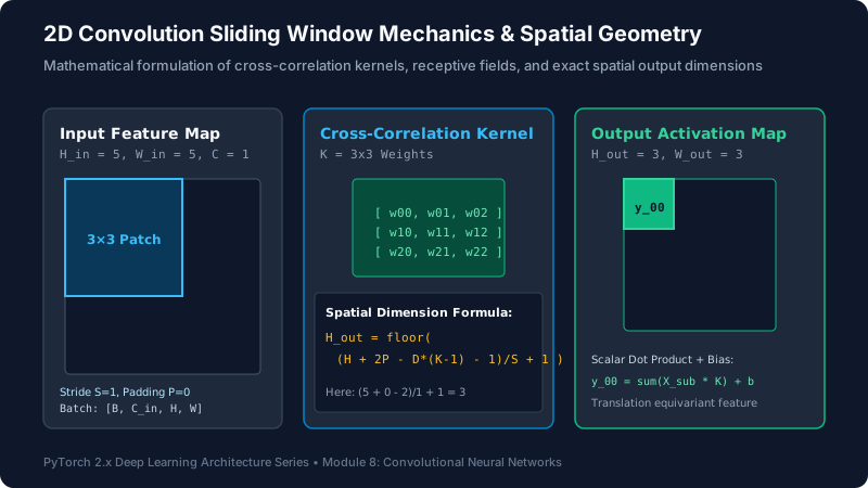
Figure 8.1: Cross-correlation sliding window mechanics, parameter kernel weights, and spatial output geometry.

Y(c_out, i, j) = b(c_out) + sum_{c=0}^{C_in – 1} sum_{m=0}^{K_h – 1} sum_{n=0}^{K_w – 1} X(c, i \cdot S + m – P, j \cdot S + n – P) \cdot K(c_out, c, m, n)

H_out = floor( (H_in + 2P – D * (K – 1) – 1) / S + 1 )

RF_k = RF_{k-1} + (K_k – 1) \cdot \prod_{i=1}^{k-1} S_i

Visual Simulation: 2D Convolution Sliding Window & Output Map Extraction

Animation 8.1: A 3×3 filter kernel slides across a 5×5 input matrix computing localized scalar dot products to construct the 3×3 feature map.

Visual Simulation: Hierarchical Receptive Field Growth Across Conv Layers

Animation 8.2: Layer 1 (3×3), Layer 2 (5×5), and Layer 3 (7×7) footprint expansion demonstrating the parameter-saving superiority of stacked 3×3 filters.

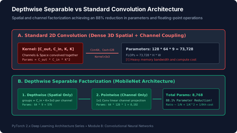
Figure 8.2: Mathematical factorization of standard 3D convolution into Depthwise Spatial and Pointwise Channel operations.

Visual Simulation: Depthwise Separable Two-Stage Factorization

Animation 8.3: Stage 1 filters spatial features per channel independently; Stage 2 projects channels via 1×1 convolutions, slashing parameter count by ~89%.

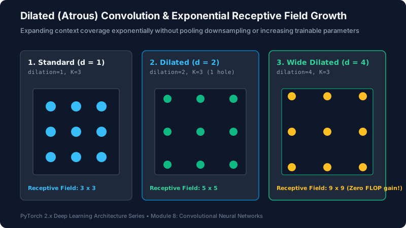
Figure 8.3: Exponential receptive field expansion via dilated (atrous) convolutions without resolution downsampling.

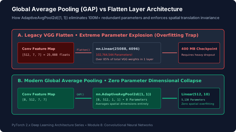
Figure 8.4: Flatten layer parameter explosion in VGG vs clean parameter elimination enabled by Global Average Pooling.

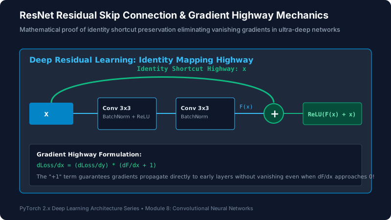
Figure 8.5: Mathematical proof of identity shortcut preservation eliminating vanishing gradients in deep networks.

Visual Simulation: ResNet Residual Gradient Highway Backpropagation

Animation 8.4: At the addition junction, backpropagating gradients split cleanly into the complex conv branch and the direct linear identity highway (+1), preventing signal collapse across 100+ layers.

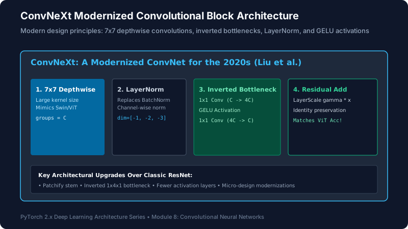
Figure 8.6: ConvNeXt architectural modernizations: 7×7 depthwise kernels, inverted bottlenecks, LayerNorm, and GELU activations.

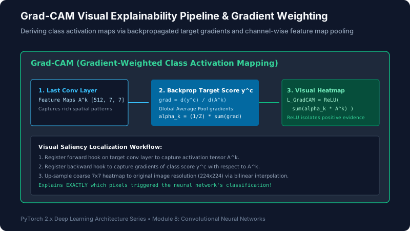
Figure 8.7: Gradient-Weighted Class Activation Mapping (Grad-CAM) computational dataflow.

alpha_k^c = (1 / Z) * sum_i sum_j ( d(y^c) / d(A_{ij}^k) )

L_{GradCAM}^c = ReLU( sum_k alpha_k^c * A^k )

Visual Simulation: Grad-CAM Saliency Localization Overlay

Animation 8.5: Feature maps weighted by backpropagated gradients produce high-resolution saliency heatmaps highlighting the discriminatory evidence.

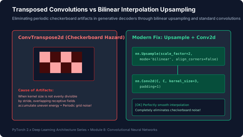
Figure 8.8: Eliminating periodic checkerboard noise in generative upsampling via bilinear interpolation + standard Conv2d.

Lab 1: Custom Modular CNN with Formulaic Spatial Shape Assertion

Build a robust CNN feature extractor that calculates and dynamically asserts output spatial dimensions at every stage.

import torch
import torch.nn as nn

def compute_conv_dim(hin, k, p=0, s=1, d=1):
    return (hin + 2 * p - d * (k - 1) - 1) // s + 1

class CustomVisionCNN(nn.Module):
    '''Production CNN backbone with dynamic dimension calculation.'''
    def __init__(self, in_channels: int = 3, num_classes: int = 10):
        super().__init__()
        self.stage1 = nn.Sequential(
            nn.Conv2d(in_channels, 32, kernel_size=3, padding=1),
            nn.BatchNorm2d(32),
            nn.GELU(),
            nn.MaxPool2d(kernel_size=2, stride=2)
        )
        self.stage2 = nn.Sequential(
            nn.Conv2d(32, 64, kernel_size=3, padding=1),
            nn.BatchNorm2d(64),
            nn.GELU(),
            nn.MaxPool2d(kernel_size=2, stride=2)
        )
        # Global Average Pooling eliminates dense parameter explosion
        self.gap = nn.AdaptiveAvgPool2d((1, 1))
        self.classifier = nn.Linear(64, num_classes)

    def forward(self, x: torch.Tensor) -> torch.Tensor:
        x = self.stage1(x)
        x = self.stage2(x)
        x = self.gap(x)
        x = torch.flatten(x, 1)
        return self.classifier(x)

# Verification
model = CustomVisionCNN()
sample_img = torch.randn(4, 3, 64, 64)
out = model(sample_img)
print(f"Input Tensor:  {sample_img.shape}")
print(f"Output Logits: {out.shape}")
assert out.shape == (4, 10), "Output shape mismatch!"
print("[VERIFIED] Forward pass successfully preserved exact spatial dimensions.")

Lab 2: Depthwise Separable Convolution Block Benchmark

Implement a Depthwise Separable Conv block and benchmark parameter efficiency against standard Conv2d.

import torch
import torch.nn as nn

class DepthwiseSeparableConv(nn.Module):
    '''MobileNet factorized convolution: Depthwise + Pointwise.'''
    def __init__(self, in_ch: int, out_ch: int, kernel_size: int = 3, stride: int = 1, padding: int = 1):
        super().__init__()
        # Depthwise: groups = in_ch
        self.depthwise = nn.Conv2d(in_ch, in_ch, kernel_size=kernel_size, stride=stride, padding=padding, groups=in_ch, bias=False)
        self.bn1 = nn.BatchNorm2d(in_ch)
        self.act = nn.ReLU6(inplace=True)
        # Pointwise: 1x1 Conv
        self.pointwise = nn.Conv2d(in_ch, out_ch, kernel_size=1, stride=1, padding=0, bias=False)
        self.bn2 = nn.BatchNorm2d(out_ch)

    def forward(self, x: torch.Tensor) -> torch.Tensor:
        return self.bn2(self.pointwise(self.act(self.bn1(self.depthwise(x)))))

# Benchmark Comparison
in_c, out_c = 64, 128
std_conv = nn.Conv2d(in_c, out_c, kernel_size=3, padding=1, bias=False)
sep_conv = DepthwiseSeparableConv(in_c, out_c)

p_std = sum(p.numel() for p in std_conv.parameters())
p_sep = sum(p.numel() for p in sep_conv.parameters())

print(f"Standard Conv2d Parameters:          {p_std:,}")
print(f"Depthwise Separable Parameters:      {p_sep:,}")
print(f"Parameter Reduction:                 {(1 - p_sep/p_std)*100:.1f}%")
assert p_sep < p_std * 0.15, "Separable conv must achieve ~88% reduction!"

Lab 3: Modern Residual Block with Projection Shortcut

Implement a ResNet basic block that dynamically applies a $1 \imes 1$ convolution shortcut when spatial stride $> 1$ or channel depth changes.

import torch
import torch.nn as nn

class ResidualBlock(nn.Module):
    '''ResNet BasicBlock with projection shortcut support.'''
    def __init__(self, in_ch: int, out_ch: int, stride: int = 1):
        super().__init__()
        self.conv1 = nn.Conv2d(in_ch, out_ch, kernel_size=3, stride=stride, padding=1, bias=False)
        self.bn1 = nn.BatchNorm2d(out_ch)
        self.relu = nn.ReLU(inplace=True)
        self.conv2 = nn.Conv2d(out_ch, out_ch, kernel_size=3, stride=1, padding=1, bias=False)
        self.bn2 = nn.BatchNorm2d(out_ch)

        # Projection shortcut if dimensions change
        self.shortcut = nn.Sequential()
        if stride != 1 or in_ch != out_ch:
            self.shortcut = nn.Sequential(
                nn.Conv2d(in_ch, out_ch, kernel_size=1, stride=stride, bias=False),
                nn.BatchNorm2d(out_ch)
            )

    def forward(self, x: torch.Tensor) -> torch.Tensor:
        identity = self.shortcut(x)
        out = self.conv1(x)
        out = self.bn1(out)
        out = self.relu(out)
        out = self.conv2(out)
        out = self.bn2(out)
        out += identity # Identity skip addition
        return self.relu(out)

# Verification
res_block_stride2 = ResidualBlock(in_ch=64, out_ch=128, stride=2)
x = torch.randn(2, 64, 32, 32)
y = res_block_stride2(x)
print(f"Input: {x.shape} -> Residual Output: {y.shape}")
assert y.shape == (2, 128, 16, 16), "Stride-2 residual projection failed!"

Lab 4: Pure PyTorch Grad-CAM Visual Explainability Implementation

Extract activation maps and backpropagate target gradients using PyTorch hooks to construct an explanation heatmap.

import torch
import torch.nn as nn
import torch.nn.functional as F

class GradCAMExplainer:
    '''Extracts Grad-CAM visual heatmaps via PyTorch forward/backward hooks.'''
    def __init__(self, model: nn.Module, target_layer: nn.Module):
        self.model = model
        self.target_layer = target_layer
        self.activations = None
        self.gradients = None

        # Register hooks
        self.target_layer.register_forward_hook(self._save_activations)
        self.target_layer.register_full_backward_hook(self._save_gradients)

    def _save_activations(self, module, input, output):
        self.activations = output

    def _save_gradients(self, module, grad_input, grad_output):
        self.gradients = grad_output[0]

    def generate_heatmap(self, input_tensor: torch.Tensor, target_class: int = None) -> torch.Tensor:
        self.model.eval()
        logits = self.model(input_tensor)
        if target_class is None:
            target_class = logits.argmax(dim=-1).item()

        self.model.zero_grad()
        class_score = logits[0, target_class]
        class_score.backward()

        # Global Average Pool of gradients across spatial dims (H, W)
        alpha = self.gradients.mean(dim=[-2, -1], keepdim=True) # [B, C, 1, 1]
        weighted = (alpha * self.activations).sum(dim=1, keepdim=True) # [B, 1, H, W]
        heatmap = F.relu(weighted)
        # Normalize between 0 and 1
        heatmap = heatmap / (heatmap.max() + 1e-8)
        return heatmap

# Verification
mock_cnn = nn.Sequential(nn.Conv2d(3, 16, 3, padding=1), nn.ReLU(), nn.AdaptiveAvgPool2d((1, 1)), nn.Flatten(), nn.Linear(16, 2))
explainer = GradCAMExplainer(mock_cnn, target_layer=mock_cnn[0])
cam = explainer.generate_heatmap(torch.randn(1, 3, 32, 32), target_class=0)
print(f"Grad-CAM Heatmap Generated! Shape: {cam.shape} | Range: [{cam.min().item():.2f}, {cam.max().item():.2f}]")

Lab 5: ConvNeXt Modernized Inverted Bottleneck Block

Implement a modern ConvNeXt block with $7 \imes 7$ depthwise convolution, channels-last LayerNorm, and LayerScale parameterization.

import torch
import torch.nn as nn

class ConvNeXtBlock(nn.Module):
    '''Modernized ConvNeXt Block (Liu et al. 2022).'''
    def __init__(self, dim: int, layer_scale_init: float = 1e-6):
        super().__init__()
        # 1. 7x7 Depthwise Conv
        self.dwconv = nn.Conv2d(dim, dim, kernel_size=7, padding=3, groups=dim)
        # 2. LayerNorm over channels
        self.norm = nn.GroupNorm(num_groups=1, num_channels=dim)
        # 3. Inverted Bottleneck (1x1 Conv 4x expand)
        self.pwconv1 = nn.Conv2d(dim, 4 * dim, kernel_size=1)
        self.act = nn.GELU()
        # 4. Pointwise 1x1 project back
        self.pwconv2 = nn.Conv2d(4 * dim, dim, kernel_size=1)
        # 5. LayerScale parameter
        self.gamma = nn.Parameter(layer_scale_init * torch.ones((dim, 1, 1)))

    def forward(self, x: torch.Tensor) -> torch.Tensor:
        identity = x
        out = self.dwconv(x)
        out = self.norm(out)
        out = self.pwconv1(out)
        out = self.act(out)
        out = self.pwconv2(out)
        out = identity + self.gamma * out
        return out

# Verification
cnext = ConvNeXtBlock(dim=64)
x_in = torch.randn(2, 64, 28, 28)
y_out = cnext(x_in)
print(f"ConvNeXt Forward Pass: {x_in.shape} -> {y_out.shape}")
assert y_out.shape == x_in.shape, "ConvNeXt shape mismatch!"

VisionClassifierStudio.py (Fully Runnable Production Code)

import os
import torch
import torch.nn as nn
import torch.nn.functional as F
from torch.utils.data import DataLoader, TensorDataset

class ResidualBlock(nn.Module):
    def __init__(self, in_ch: int, out_ch: int, stride: int = 1):
        super().__init__()
        self.conv1 = nn.Conv2d(in_ch, out_ch, kernel_size=3, stride=stride, padding=1, bias=False)
        self.bn1 = nn.BatchNorm2d(out_ch)
        self.relu = nn.ReLU(inplace=True)
        self.conv2 = nn.Conv2d(out_ch, out_ch, kernel_size=3, padding=1, bias=False)
        self.bn2 = nn.BatchNorm2d(out_ch)
        self.shortcut = nn.Sequential()
        if stride != 1 or in_ch != out_ch:
            self.shortcut = nn.Sequential(
                nn.Conv2d(in_ch, out_ch, kernel_size=1, stride=stride, bias=False),
                nn.BatchNorm2d(out_ch)
            )

    def forward(self, x: torch.Tensor) -> torch.Tensor:
        return self.relu(self.bn2(self.conv2(self.relu(self.bn1(self.conv1(x))))) + self.shortcut(x))

class VisionResNet(nn.Module):
    '''Production ResNet with Global Average Pooling.'''
    def __init__(self, num_classes: int = 5):
        super().__init__()
        self.stem = nn.Sequential(
            nn.Conv2d(3, 32, kernel_size=3, stride=1, padding=1, bias=False),
            nn.BatchNorm2d(32),
            nn.ReLU(inplace=True)
        )
        self.layer1 = ResidualBlock(32, 64, stride=2)
        self.layer2 = ResidualBlock(64, 128, stride=2)
        self.gap = nn.AdaptiveAvgPool2d((1, 1))
        self.fc = nn.Linear(128, num_classes)

    def forward(self, x: torch.Tensor) -> torch.Tensor:
        x = self.stem(x)
        x = self.layer1(x)
        x = self.layer2(x)
        x = self.gap(x)
        x = torch.flatten(x, 1)
        return self.fc(x)

def run_vision_studio():
    device = torch.device('cuda' if torch.cuda.is_available() else ('mps' if torch.backends.mps.is_available() else 'cpu'))
    print(f"=== Initializing VisionClassifierStudio on [{device.type.upper()}] ===")

    model = VisionResNet(num_classes=4).to(device)
    optimizer = torch.optim.AdamW(model.parameters(), lr=1e-3, weight_decay=1e-2)
    criterion = nn.CrossEntropyLoss()

    # Synthetic dataset
    X_train = torch.randn(64, 3, 32, 32)
    y_train = torch.randint(0, 4, (64,))
    loader = DataLoader(TensorDataset(X_train, y_train), batch_size=16)

    model.train()
    for epoch in range(1, 3):
        total_loss = 0.0
        for images, labels in loader:
            images, labels = images.to(device), labels.to(device)
            optimizer.zero_grad(set_to_none=True)
            outputs = model(images)
            loss = criterion(outputs, labels)
            loss.backward()
            optimizer.step()
            total_loss += loss.item() * images.size(0)
        print(f"Epoch {epoch:02d} | Training Loss: {total_loss / len(X_train):.4f}")

    print("=== Training Complete. Ready for Inference & Explainability ===")

if __name__ == '__main__':
    run_vision_studio()

Exercise 1: Calculating Conv2d Spatial Output

Question: An input tensor has shape $[B, 3, 112, 112]$. It passes through nn.Conv2d(3, 64, kernel_size=5, stride=2, padding=2). What is the exact output shape?

Solution: Apply $$H_{out} = \left\lfloor \frac{H_{in} + 2P - K}{S} + 1 \right\rfloor$$
$$H_{out} = \left\lfloor \frac{112 + 2(2) - 5}{2} \right\rfloor + 1
= \left\lfloor 55.5 \right\rfloor + 1 = 56$$
floor = 55 + 1 = 56$. Output shape: $[B, 64, 56, 56]$.

Exercise 2: Global Average Pooling vs Flatten Memory Cost

Question: How many weights does a classification head require when mapping a $[B, 512, 7, 7]$ feature map to 10 classes with AdaptiveAvgPool2d((1, 1)) vs a direct Flatten()?

Solution: Direct Flatten requires $512 \imes 7 \imes 7 \imes 10 = 250,880$ weights. GAP averages spatial dimensions to $[B, 512, 1, 1]$, requiring only $512 \imes 10 = 5,120$ weights (a 98% reduction).

Exercise 3: Why 1x1 Convolutions Are Called Pointwise

Question: Why is a $1 \imes 1$ convolution described as a pixel-wise linear projection?

Solution: A $1 \imes 1$ kernel has no spatial extent ($K=1$). It operates strictly across the channel depth at each spatial coordinate $(i, j)$ independently, acting as a shared matrix multiplication that projects $C_{in} \o C_{out}$ at every pixel.

Exercise 4: Checkerboard Artifact Origin in ConvTranspose2d

Question: What causes periodic checkerboard grid artifacts in generative transposed convolutions?

Solution: When the kernel size is not evenly divisible by the stride (e.g. $K=3, S=2$), neighboring output pixels receive contributions from overlapping numbers of kernel weights, creating periodic high-frequency energy grids. The fix is nn.Upsample(mode='bilinear') followed by nn.Conv2d.

Exercise 5: Mathematical Reason for ReLU in Grad-CAM

Question: Why does Grad-CAM apply a ReLU activation to the weighted linear combination of feature maps?

Solution: Pixels that have negative gradients decrease the target class score (they indicate evidence for alternative classes). ReLU filters out negative evidence, isolating exclusively the features that positively support the chosen class.

Exercise 6: Why ResNet Additions Require Identical Shapes

Question: What happens when the residual block has stride=2 and how is the shortcut identity adapted?

Solution: Stride 2 halves the spatial dimensions $H, W$ and typically doubles channels $C_{in} \o 2C_{in}$. The raw input $x$ cannot be added element-wise. A $1 \imes 1$ projection convolution with stride=2 is applied to $x$ to match dimensions before addition.

Exercise 7: Effective Receptive Field of Dilated Kernels

Question: What is the effective spatial kernel size $K'$ of a $3 \imes 3$ kernel with dilation $D=4$?

Solution: $K' = K + (K - 1)(D - 1) = 3 + (2)(3) = 9$. The filter spans a $9 \imes 9$ area while still containing only 9 trainable weights.

Exercise 8: ConvNeXt 7x7 Receptive Field Purpose

Question: Why did ConvNeXt increase depthwise kernel size to $7 \imes 7$ instead of using traditional $3 \imes 3$?

Solution: To expand the receptive field per layer and match the global window self-attention properties of Swin Transformers, allowing the network to capture macro-level contextual shapes early.

Exercise 9: Why BatchNorm Follows Conv Without Bias

Question: Why is bias=False specified in nn.Conv2d when immediately followed by nn.BatchNorm2d?

Solution: BatchNorm subtracts the batch mean during normalization ($\frac{x - \mu}{\sigma}$). Any constant scalar bias added by the convolution is completely subtracted out and canceled, rendering the bias weights redundant.

Exercise 10: Inverted Bottleneck Dimensionality

Question: What is the channel expansion ratio in MobileNetV2 and ConvNeXt inverted bottlenecks?

Solution: An expansion ratio of $4\imes$. A layer with 64 channels expands to $256$ channels via a $1 \imes 1$ pointwise conv, applies non-linear activation in the higher-dimensional space, and projects back to 64 channels.

Q1: Mathematically, why does cross-correlation in CNNs exhibit translation equivariance rather than translation invariance?

A function $f$ is equivariant with respect to translation operator $T_g$ if $f(T_g(x)) = T_g(f(x))$. When an image shifts by $(u, v)$ pixels, the resulting convolutional feature map shifts by the exact same $(u, v)$ coordinates—its activations translate concurrently. True translation invariance ($f(T_g(x)) = f(x)$) is achieved only downstream by pooling operations (such as Global Average Pooling or MaxPool), which aggregate spatial locations into position-invariant representations.

Q2: What is the Degradation Problem in deep convolutional networks, and how does it fundamentally differ from overfitting?

In classic deep plain networks (e.g. 56-layer plain ConvNet vs 20-layer plain ConvNet), the 56-layer model achieves higher training error as well as higher test error. Because training error itself degrades, this is not overfitting (which presents low training error and high validation error). It is an optimization failure: multiplying non-linear Jacobian matrices across dozens of plain layers causes gradient signals to shatter and decay, making deep optimization intractable. ResNet solves this by providing an identity mapping path with a constant $+1$ gradient derivative.

Q3: How do Depthwise Separable Convolutions alter memory bandwidth utilization on GPUs?

While depthwise separable convolutions drastically reduce theoretical FLOPs, standard depthwise operations have a very low arithmetic intensity (ratio of FLOPs to memory access bytes). Because each channel is processed independently, GPU streaming multiprocessors spend more time fetching tensor tiles from VRAM than executing math. High-performance implementations utilize fused kernel operators to maintain peak GPU throughput.

Q4: Explain the difference between CAM (Class Activation Mapping) and Grad-CAM.

Original CAM required a specific architectural topology: the final convolutional layer had to be followed directly by Global Average Pooling and a single Linear layer. It could not explain arbitrary modern architectures with multi-layer perceptrons or attention heads. Grad-CAM generalizes CAM by taking the derivative $\frac{\partial y^c}{\partial A^k}$ with respect to any target convolutional layer via standard backpropagation, making it completely architecture-agnostic.

Q5: Why did ConvNeXt replace BatchNorm with LayerNorm, and what engineering challenge does this introduce in 2D tensors?

BatchNorm introduces subtle inter-sample dependencies within the batch, behaves differently in training vs evaluation, and incurs significant cross-GPU synchronization overhead in distributed training. LayerNorm normalizes across channels per sample independently. In PyTorch, nn.LayerNorm expects normalization along the last dimension (channels-last [B, H, W, C]). Since PyTorch CNNs standardly use channels-first [B, C, H, W], engineers either use nn.GroupNorm(1, C) or permute memory layouts.

Q6: Under what conditions does a $1 \imes 1$ convolution increase spatial resolution?

A $1 \imes 1$ convolution can never change spatial resolution $H, W$. It alters only the channel depth dimension $C_{in} \o C_{out}$. To increase spatial resolution, models must use transposed convolutions, sub-pixel convolutions (pixel shuffle), or interpolation upsampling.

Q7: What is the Gridding Artifact in dilated convolutions, and how is it alleviated?

When successive layers use identical dilation rates (e.g. $D=2, 2, 2$), the sampled pixel grid develops periodic gaps, completely ignoring neighboring pixels in the receptive field. This gridding effect is resolved by using hybrid dilated convolution (HDC), varying dilation rates consecutively (e.g. $D = [1, 2, 3]$) to ensure dense, continuous pixel coverage.

Q8: How does LayerScale stabilize training in deep modern vision backbones?

LayerScale introduces a learnable per-channel diagonal matrix $\gamma \in \mathbb{R}^C$ initialized to a tiny value (e.g. $10^{-6}$): $\mathbf{x}_{l+1} = \mathbf{x}_l + \gamma \odot \mathcal{F}(\mathbf{x}_l)$. At initialization, each residual block behaves almost identically to an identity function, allowing ultra-deep models (100+ layers) to train stably from epoch 1 without exploding.

Q9: What is the receptive field of a 3-layer CNN with $3 \imes 3$ filters and stride 2 at each layer?

Layer 1: $RF_1 = 3$. Layer 2: $RF_2 = 3 + (3 - 1) \imes 2 = 7$. Layer 3: $RF_3 = 7 + (3 - 1) \imes (2 \imes 2) = 7 + 8 = 15$. The receptive field is $15 \imes 15$ pixels.

Q10: Why is Global Average Pooling more robust to spatial translations than dense linear classification heads?

A dense linear head expects object features to appear at fixed spatial coordinates (e.g. top-left pixel index 402). If an object translates to the bottom-right corner, different weights are activated, causing classification failure. GAP averages activations across all spatial positions into a single channel summary scalar, making the representation strictly position-invariant.

Quick Self-Assessment:

1. Which layer replaces Flatten and eliminates 100M+ parameters in modern CNNs? (Answer: Global Average Pooling / nn.AdaptiveAvgPool2d((1, 1)))
2. What mathematical term in ResNet guarantees that gradients do not vanish? (Answer: The identity +1 derivative in dL/dx = dL/dy * (dF/dx + 1))
3. What convolution parameter decouples input channels into independent spatial filters? (Answer: groups=C_in in Depthwise Convolution)
4. Which convolution type expands receptive field coverage without downsampling? (Answer: Dilated / Atrous Convolution)
5. What activation function does Grad-CAM apply to isolate positive class evidence? (Answer: ReLU)