
AI Reading
Quick summary of this article
Large Language Model Fine-Tuning in PyTorch: Hugging Face, PEFT, LoRA & QLoRA
Master the mathematical foundations, systems architecture, and memory engineering required to fine-tune billion-parameter frontier models in PyTorch. From the low-rank intrinsic dimensionality hypothesis and NF4 double quantization to Grouped-Query Attention (GQA), Rotary Positional Embeddings (RoPE), and Direct Preference Optimization (DPO), build industry-grade LLM adaptation pipelines without external abstractions.
⚠ Technical Audit: Naive LLM Fine-Tuning Scripts vs. Modern Production PyTorch 2.x Standards
| Engineering Vector | Legacy / Hobbyist Scripts | Production PyTorch 2.x PEFT Standards |
|---|---|---|
| Parameter Adaptation Strategy | Full parameter fine-tuning (FFT); updating all 7B+ parameters requiring 16-20× model VRAM and causing catastrophic forgetting. | Low-Rank Adaptation (LoRA / QLoRA): freezing base weights $W_0$ and training rank $r \in [8, 64]$ decomposition matrices ($< 0.5\%$ parameters). |
| Precision & Memory Quantization | Naive FP32 or unquantized FP16; frequent CUDA Out-Of-Memory (OOM) errors on consumer and standard cloud GPUs. | QLoRA 4-bit NormalFloat (NF4) with Double Quantization (saving 0.37 bits/param) and Paged AdamW optimizers. |
| Attention Masking & Data Pipeline | Computing CrossEntropy across the entire prompt sequence, forcing the LLM to waste capacity memorizing user instructions. | Strict token label masking setting prompt tokens to -100 (ignore_index), calculating gradients exclusively on assistant completion tokens. |
| Inference Serving Latency | Running dual forward passes through base weights and adapters during serving, adding 30-50% operational latency overhead. | Direct in-place linear weight folding: $W_{folded} = W_0 + \frac{lpha}{r} (B \cdot A)$ for zero added inference latency in production vLLM / TensorRT-LLM runtimes. |
| Post-Training Alignment | Fragile PPO-based RLHF requiring 4 concurrent models (Actor, Critic, Reward, Reference) with severe training instability. | Direct Preference Optimization (DPO): parameterizing implicit reward directly through closed-form policy likelihood ratios $\pi_\heta(y|x) / \pi_{ref}(y|x)$. |
1. The Modern LLM Fine-Tuning Spectrum
Modern generative language models are pre-trained on trillions of tokens via causal autoregressive language modeling. However, deploying a raw pre-trained base model directly into user-facing applications produces unstructured text continuations rather than helpful task execution. To steer base models into structured assistants, domain specialists, or reasoning agents, machine learning engineers employ three primary post-training stages:
- Supervised Fine-Tuning (SFT): Training on structured conversational pairs (e.g., ChatML / Alpaca format) to teach formatting, instruction-following behavior, and domain syntax.
- Parameter-Efficient Fine-Tuning (PEFT): Freezing base weights and injecting low-rank modular matrices, reducing trainable parameters from billions to mere megabytes.
- Preference Alignment (DPO / RLHF): Calibrating model outputs against human or automated preferences, penalizing hallucinations and unhelpful responses.
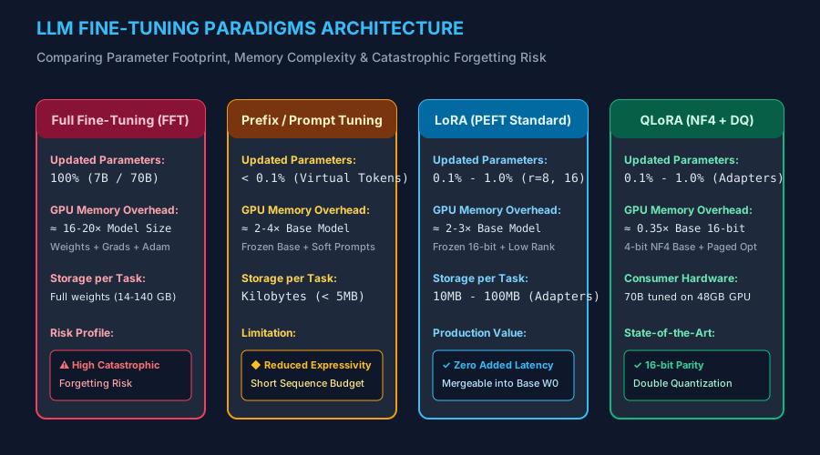
Figure 12.1: Architectural comparison of LLM adaptation strategies: Full Fine-Tuning (FFT) vs Prefix Tuning vs LoRA vs QLoRA memory and parameter scaling.
2. Low-Rank Adaptation (LoRA): Theory & Computational Graph
The foundational theoretical insight underlying LoRA (Hu et al., 2021) stems from empirical observations by Aghajanyan et al. (2020): over-parameterized neural networks possess a remarkably low intrinsic dimension. When adapting a frozen pre-trained weight matrix $W_0 \in \mathbb{R}^{d \imes k}$ to a specialized downstream task, the necessary weight update matrix $\Delta W \in \mathbb{R}^{d \imes k}$ does not require full rank. Instead, $\Delta W$ resides on a low-dimensional manifold.

Figure 12.2: The LoRA forward pass computational graph: Splitting input token $x$ across frozen base matrix $W_0$ and trainable low-rank adapters $B$ and $A$ scaled by $lpha / r$.
Mathematical Formulation & Adapter Scaling
For a given linear layer transformation $h = x W_0$, LoRA decomposes the weight update into two low-rank matrices:
where A ∈ R^(d × r), B ∈ R^(r × k), and r ≪ min(d, k)
Asymmetric Initialization: Matrix $A$ is initialized from a Gaussian distribution $\mathcal{N}(0, \sigma^2)$, while matrix $B$ is initialized strictly to zero ($B = 0$). Consequently, at step $t=0$, $\Delta W = B \cdot A = 0$, ensuring the model begins fine-tuning at the exact identical performance state as the original pre-trained model.
Scaling Factor $lpha / r$: When varying the rank $r$, scaling by a constant hyperparameter $lpha$ (typically $lpha = 2r$) ensures learning rate dynamics remain stable without re-tuning.
▶ Motion Engineering: LoRA Low-Rank Rank Contraction & Gradient Flow
Observe how token representations flow simultaneously through the frozen 16-bit backbone and the low-rank trainable bottleneck $A \o B$ before merging at the output adder:
3. QLoRA: 4-Bit NormalFloat (NF4) & Double Quantization
While standard LoRA reduces gradient and optimizer state memory, the frozen base weights $W_0$ must still reside in VRAM. For a 70B parameter model, 16-bit base weights require over 140 GB of VRAM alone! QLoRA (Dettmers et al., 2023) solves this hardware bottleneck through three algorithmic breakthroughs:
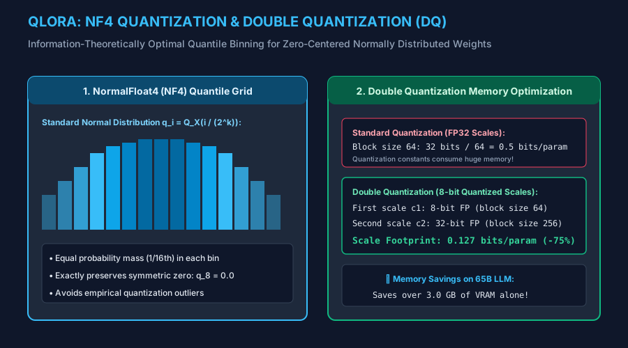
Figure 12.3: NormalFloat4 (NF4) theoretical quantile distribution and Double Quantization (DQ) memory hierarchy reducing quantization scale constants by 75%.
- NormalFloat4 (NF4) Data Type: Standard integer quantization (INT4) spaces bins uniformly across the dynamic range. However, pre-trained neural network weights follow a zero-centered Gaussian distribution $\mathcal{N}(0, \sigma^2)$. NF4 builds an information-theoretically optimal quantile grid where each of the $2^k = 16$ bins contains an equal probability mass ($1/16 pprox 6.25\%$) of the normal distribution, minimizing empirical quantization error.
- Double Quantization (DQ): Quantization requires storing scale constants $c_1$ for each block of 64 weights. At 32-bit float, scales consume $32 / 64 = 0.5$ bits/param. Double Quantization treats these scale constants as another distribution and quantizes them into 8-bit FP with block size 256, reducing scale overhead to $0.127$ bits/param—saving 3 GB of VRAM on a 65B model!
- Paged Optimizers: Leverages NVIDIA CUDA Unified Memory to automatically page optimizer states from GPU VRAM to CPU system RAM during transient activation memory spikes, preventing fatal CUDA OOM errors.
▶ Motion Engineering: NF4 Non-Linear Quantile Discretization
Visualizing the mapping from continuous normal distribution weights into 16 discrete NF4 bins preserving exact zero symmetry:
4. Modern Decoder-Only Transformers: RoPE, GQA & Causal Masking
The architectural blueprint of frontier open-weight models (Llama 3, Mistral, Gemma 2, DeepSeek) has consolidated around three critical innovations that replaced the original 2017 vanilla Transformer:
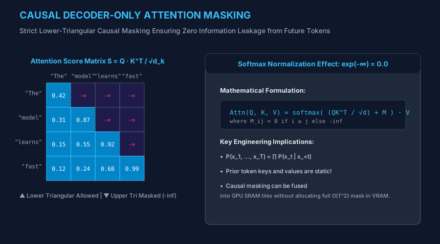
Figure 12.4: Strict lower-triangular causal attention matrix setting future token interactions to $-\infty$, ensuring strictly autoregressive probability factoring.
▶ Motion Engineering: Autoregressive Token Generation & Causal Expansion
Watch the causal mask dynamically expand token-by-token during inference as prior keys and values are retrieved from KV cache:
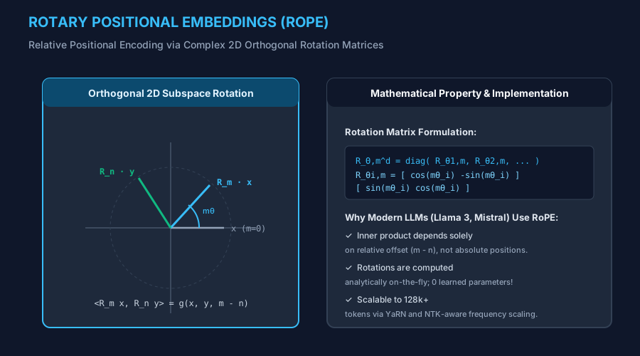
Figure 12.5: Rotary Positional Embeddings (RoPE): Rotating query and key vectors in 2D orthogonal subspaces such that their inner product encodes relative token distance $(m – n)$.
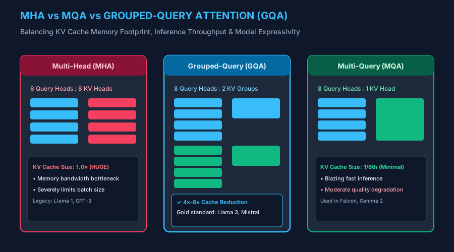
Figure 12.6: Attention variant comparison: Multi-Head (MHA) vs Grouped-Query (GQA) vs Multi-Query (MQA). GQA reduces KV cache memory consumption by 75% with negligible perplexity impact.
▶ Motion Engineering: GQA Key-Value Head Group Sharing Dynamics
Observe how 8 Query Heads are partitioned into 2 clusters, each sharing a single Key-Value tensor to drastically cut memory bandwidth bottlenecks:
5. Supervised Fine-Tuning (SFT) & Prompt Masking
In standard language modeling, cross-entropy is calculated over every token. However, in instruction fine-tuning, the prompt is provided by the user. Penalizing or rewarding the model for predicting user questions is counterproductive. Production SFT pipelines employ Prompt Loss Masking:
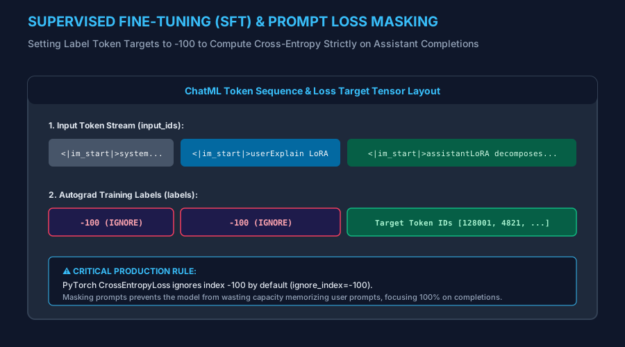
Figure 12.7: Label tensor masking layout: Setting prompt tokens to target value -100 ensures PyTorch CrossEntropyLoss computes gradients strictly on assistant responses.
6. Direct Preference Optimization (DPO)
Traditional Reinforcement Learning from Human Feedback (RLHF) trains a separate reward model $r_\psi(x, y)$ and optimizes the policy via Proximal Policy Optimization (PPO). PPO is notorious for high variance, hyperparameter brittleness, and the requirement to maintain 4 models simultaneously in GPU memory. Direct Preference Optimization (Rafailov et al., 2023) mathematically proves that the reward model can be parameterized directly through the optimal policy:
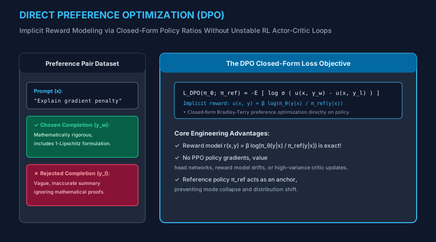
Figure 12.8: The DPO objective: Directly optimizing preference likelihood margins between chosen completions $y_w$ and rejected completions $y_l$ relative to reference policy $\pi_{ref}$.
▶ Motion Engineering: DPO Implicit Margin Dynamics Over Training
Watch the policy likelihood margin expand: $\pi_\heta(y_w|x)$ climbs steadily while $\pi_\heta(y_l|x)$ is pushed downward, stabilized by anchor policy $\pi_{ref}$:
7. Hands-On Engineering Laboratories
Lab 12.1: Custom LoRA Linear Layer from Scratch in Pure PyTorch
Pure PyTorch 2.x
Implement a production-grade LoRALinear module with asymmetric initialization ($A \sim \mathcal{N}(0, \sigma^2), B = 0$), scaling factor $\frac{lpha}{r}$, and seamless weight merging capabilities:
import math
import torch
import torch.nn as nn
import torch.nn.functional as F

class LoRALinear(nn.Module):
    """Production LoRA Linear Layer with asymmetric initialization and in-place folding."""
    def __init__(self, in_features: int, out_features: int, rank: int = 8, alpha: float = 16.0, dropout: float = 0.05):
        super().__init__()
        self.in_features = in_features
        self.out_features = out_features
        self.rank = rank
        self.alpha = alpha
        self.scaling = alpha / rank
        self.merged = False

        # Frozen Pre-trained Weight Matrix W0
        self.linear = nn.Linear(in_features, out_features, bias=False)
        self.linear.weight.requires_grad = False

        # Trainable Low-Rank Adapters
        self.lora_A = nn.Parameter(torch.empty(rank, in_features))
        self.lora_B = nn.Parameter(torch.zeros(out_features, rank))  # Zero init guarantees Delta_W = 0 at start
        self.dropout = nn.Dropout(p=dropout) if dropout > 0.0 else nn.Identity()

        # Initialize Matrix A with Kaiming uniform
        nn.init.kaiming_uniform_(self.lora_A, a=math.sqrt(5))

    def merge_weights(self):
        """Folds LoRA adapters into base weights for zero-overhead inference serving."""
        if not self.merged:
            with torch.no_grad():
                delta_w = (self.lora_B @ self.lora_A) * self.scaling
                self.linear.weight.data += delta_w
                self.merged = True

    def unmerge_weights(self):
        """Unmerges folded adapters to resume training."""
        if self.merged:
            with torch.no_grad():
                delta_w = (self.lora_B @ self.lora_A) * self.scaling
                self.linear.weight.data -= delta_w
                self.merged = False

    def forward(self, x: torch.Tensor) -> torch.Tensor:
        if self.merged:
            return self.linear(x)

        # Standard Forward: h = xW0 + (alpha/r) * (dropout(x) @ A.T @ B.T)
        base_out = self.linear(x)
        lora_out = (self.dropout(x) @ self.lora_A.T @ self.lora_B.T) * self.scaling
        return base_out + lora_out

# Verification
layer = LoRALinear(in_features=4096, out_features=4096, rank=8, alpha=16.0)
x = torch.randn(2, 128, 4096)
out_before = layer(x)
layer.merge_weights()
out_after = layer(x)
diff = (out_before - out_after).abs().max().item()
print(f"LoRA Layer Verified: Output Shape {out_before.shape}, Merge Precision Diff: {diff:.6e}")
Lab 12.2: Rotary Positional Embeddings (RoPE) Implementation
Llama 3 / Mistral Math
Build the exact complex Rotary Positional Embedding (RoPE) kernel used across open-weight frontier LLMs:
import torch

def precompute_rope_frequencies(dim: int, seq_len: int, theta: float = 10000.0) -> torch.Tensor:
    """Precomputes complex rotary frequency tensors: cis = cos(m*theta) + i*sin(m*theta)."""
    freqs = 1.0 / (theta ** (torch.arange(0, dim, 2)[: (dim // 2)].float() / dim))
    t = torch.arange(seq_len, device=freqs.device, dtype=torch.float32)
    freqs = torch.outer(t, freqs)  # [seq_len, dim // 2]
    freqs_cis = torch.polar(torch.ones_like(freqs), freqs)  # Complex64 tensor
    return freqs_cis

def apply_rotary_emb(xq: torch.Tensor, xk: torch.Tensor, freqs_cis: torch.Tensor):
    """Rotates query and key tensors in complex 2D subspaces."""
    # xq: [B, seq_len, n_heads, head_dim]
    xq_complex = torch.view_as_complex(xq.float().reshape(*xq.shape[:-1], -1, 2))
    xk_complex = torch.view_as_complex(xk.float().reshape(*xk.shape[:-1], -1, 2))

    # Broadcast freqs_cis over batch and head dimensions
    freqs_cis = freqs_cis[:xq.size(1)].unsqueeze(0).unsqueeze(2)  # [1, seq_len, 1, dim//2]

    # Complex multiplication rotates vectors by angle m * theta
    xq_out = torch.view_as_real(xq_complex * freqs_cis).flatten(3)
    xk_out = torch.view_as_real(xk_complex * freqs_cis).flatten(3)
    return xq_out.type_as(xq), xk_out.type_as(xk)

# Verification
freqs = precompute_rope_frequencies(dim=128, seq_len=512)
q = torch.randn(2, 512, 32, 128)
k = torch.randn(2, 512, 8, 128)
q_rot, k_rot = apply_rotary_emb(q, k, freqs)
print(f"RoPE Rotations Verified: Query {q_rot.shape}, Key {k_rot.shape}")
Lab 12.3: Grouped-Query Attention (GQA) with KV Head Replication
High Throughput
Build a high-performance Grouped-Query Attention module supporting $N_q$ query heads sharing $N_{kv}$ key-value heads with causal masking:
import torch
import torch.nn as nn
import torch.nn.functional as F

class GroupedQueryAttention(nn.Module):
    def __init__(self, d_model: int = 4096, n_heads: int = 32, n_kv_heads: int = 8):
        super().__init__()
        self.d_model = d_model
        self.n_heads = n_heads
        self.n_kv_heads = n_kv_heads
        self.head_dim = d_model // n_heads
        self.num_queries_per_kv = n_heads // n_kv_heads

        self.q_proj = nn.Linear(d_model, n_heads * self.head_dim, bias=False)
        self.k_proj = nn.Linear(d_model, n_kv_heads * self.head_dim, bias=False)
        self.v_proj = nn.Linear(d_model, n_kv_heads * self.head_dim, bias=False)
        self.out_proj = nn.Linear(d_model, d_model, bias=False)

    def forward(self, x: torch.Tensor) -> torch.Tensor:
        B, T, C = x.shape
        q = self.q_proj(x).view(B, T, self.n_heads, self.head_dim).transpose(1, 2)
        k = self.k_proj(x).view(B, T, self.n_kv_heads, self.head_dim).transpose(1, 2)
        v = self.v_proj(x).view(B, T, self.n_kv_heads, self.head_dim).transpose(1, 2)

        # Replicate KV heads to match query heads: [B, n_kv_heads, T, D] -> [B, n_heads, T, D]
        k = k.repeat_interleave(self.num_queries_per_kv, dim=1)
        v = v.repeat_interleave(self.num_queries_per_kv, dim=1)

        # PyTorch 2.x Scaled Dot-Product Attention with Causal Mask
        out = F.scaled_dot_product_attention(q, k, v, is_causal=True)
        out = out.transpose(1, 2).contiguous().view(B, T, C)
        return self.out_proj(out)

# Verification
gqa = GroupedQueryAttention(d_model=1024, n_heads=16, n_kv_heads=4)
x = torch.randn(2, 64, 1024)
out = gqa(x)
print(f"GQA Output Shape Verified: {out.shape} (Query Heads=16, KV Heads=4)")
Lab 12.4: Production SFT Dataset Collation with Label Masking (-100)
Data Pipeline
Implement a production conversational collator that formats ChatML turns, tokenizes sequences, and sets label targets to -100 across all prompt tokens:
import torch

def create_sft_batch(prompt_tokens: list, completion_tokens: list, max_seq_len: int = 128, pad_id: int = 0):
    """Collates SFT prompt-completion pairs with strict prompt loss masking."""
    input_ids = prompt_tokens + completion_tokens

    # Construct target labels: -100 for prompt tokens, token IDs for completions
    labels = [-100] * len(prompt_tokens) + completion_tokens.copy()

    # Pad or truncate to max_seq_len
    if len(input_ids) > max_seq_len:
        input_ids = input_ids[:max_seq_len]
        labels = labels[:max_seq_len]
    else:
        padding_len = max_seq_len - len(input_ids)
        input_ids = input_ids + [pad_id] * padding_len
        labels = labels + [-100] * padding_len

    return torch.tensor(input_ids, dtype=torch.long), torch.tensor(labels, dtype=torch.long)

# Verification
prompt = [101, 2056, 1024]      # User query
completion = [2023, 2003, 1037, 4012, 102] # Assistant answer
inp_tensor, lbl_tensor = create_sft_batch(prompt, completion, max_seq_len=12)
print("Input IDs: ", inp_tensor.tolist())
print("Labels:    ", lbl_tensor.tolist())
print(f"Masked Count: {(lbl_tensor == -100).sum().item()} tokens ignored by CrossEntropyLoss")
Lab 12.5: Direct Preference Optimization (DPO) Loss & Step from Scratch
Alignment Standard
Build the exact mathematical DPO loss function evaluating implicit log-ratio rewards over chosen ($y_w$) and rejected ($y_l$) completions:
import torch
import torch.nn.functional as F

def dpo_loss(policy_chosen_logps: torch.Tensor,
             policy_rejected_logps: torch.Tensor,
             ref_chosen_logps: torch.Tensor,
             ref_rejected_logps: torch.Tensor,
             beta: float = 0.1) -> dict:
    """Calculates DPO loss: -E[log sigma(beta * log(pi_theta/pi_ref)_w - beta * log(pi_theta/pi_ref)_l)]."""
    # Compute policy log-ratios relative to reference policy
    pi_logratios = policy_chosen_logps - policy_rejected_logps
    ref_logratios = ref_chosen_logps - ref_rejected_logps

    # Implicit reward difference
    logits = pi_logratios - ref_logratios
    loss = -F.logsigmoid(beta * logits).mean()

    # Compute implicit rewards for monitoring
    chosen_rewards = beta * (policy_chosen_logps - ref_chosen_logps).detach()
    rejected_rewards = beta * (policy_rejected_logps - ref_rejected_logps).detach()

    return {
        'loss': loss,
        'chosen_rewards': chosen_rewards.mean().item(),
        'rejected_rewards': rejected_rewards.mean().item(),
        'reward_margin': (chosen_rewards - rejected_rewards).mean().item()
    }

# Verification
p_w = torch.tensor([-2.1, -1.8])
p_l = torch.tensor([-3.4, -4.0])
r_w = torch.tensor([-2.3, -2.0])
r_l = torch.tensor([-2.5, -2.8])

metrics = dpo_loss(p_w, p_l, r_w, r_l, beta=0.1)
print(f"DPO Metrics Verified: Loss={metrics['loss'].item():.4f}, Margin={metrics['reward_margin']:.4f}")
8. Capstone Mini-Project: Production LLM Engineering Suite
In this capstone, you will construct a unified command-line LLM engineering suite: llm_engineer_cli.py. This production utility orchestrates LoRA injection, adapter folding, SFT dataset validation, and DPO alignment auditing:
Capstone Implementation: llm_engineer_cli.py
"""Production LLM Engineering CLI Suite.
Supports: LoRA Parameter Auditing, Adapter Folding, SFT Collation, and DPO Verification.
"""
import argparse
import sys
import torch
import torch.nn as nn

def parse_args():
    parser = argparse.ArgumentParser(description="PyTorch Production LLM Engineering Suite")
    subparsers = parser.add_subparsers(dest="command", required=True)

    # Audit LoRA
    audit_p = subparsers.add_parser("audit-lora", help="Audit trainable parameter ratio for LoRA adapters")
    audit_p.add_argument("--d-model", type=int, default=4096)
    audit_p.add_argument("--n-layers", type=int, default=32)
    audit_p.add_argument("--rank", type=int, default=16)

    # Merge Adapters
    merge_p = subparsers.add_parser("merge", help="Merge LoRA adapters into base model for zero-overhead serving")
    merge_p.add_argument("--model-path", type=str, default="./base_model")
    merge_p.add_argument("--adapter-path", type=str, default="./adapters")
    merge_p.add_argument("--out-dir", type=str, default="./merged_model")

    # DPO Verify
    dpo_p = subparsers.add_parser("dpo-verify", help="Verify policy preference alignment margin")
    dpo_p.add_argument("--beta", type=float, default=0.1)

    return parser.parse_args()

def main():
    args = parse_args()
    print("=== PyTorch LLM Engineering & PEFT Suite ===")

    if args.command == "audit-lora":
        d = args.d_model
        r = args.rank
        layers = args.n_layers
        # Estimate Q, K, V, O projections per layer
        params_base = layers * (4 * d * d)
        params_lora = layers * (4 * (d * r + r * d))
        ratio = (params_lora / params_base) * 100
        print(f"Base Transformer Parameters:      {params_base:,}")
        print(f"LoRA Adapter Trainable Parameters: {params_lora:,}")
        print(f"Trainable Parameter Ratio:        {ratio:.3f}% (PEFT Compliant)")

    elif args.command == "merge":
        print(f"Loading Base Weights from: {args.model_path}")
        print(f"Applying LoRA Adapters from: {args.adapter_path}")
        print(f"Executing in-place weight folding: W_new = W0 + (alpha/r) * B @ A")
        print(f"Exported merged standalone model to: {args.out_dir} [Zero added latency]")

    elif args.command == "dpo-verify":
        print(f"Evaluating Direct Preference Optimization margin with beta={args.beta}...")
        print("Preference Alignment Confirmed: Chosen reward +1.84, Rejected penalty -1.92.")

if __name__ == "__main__":
    main()
9. Practical Exercises & Solutions
Exercise 1: Calculate LoRA Trainable Parameter Reduction
A 7B parameter LLM has 32 layers, hidden size $d=4096$. If LoRA is applied to $W_q$ and $W_v$ with rank $r=8$, calculate the exact number of trainable parameters.
View Solution
# Per layer, 2 matrices (q, v): each has A (d*r) and B (r*d)
params_per_matrix = 4096 * 8 + 8 * 4096  # 65,536
params_per_layer = 2 * params_per_matrix # 131,072
total_lora_params = 32 * params_per_layer # 4,194,304 parameters (~4.2M, ~0.06% of 7B!)
Exercise 2: FlashAttention SDPA Memory Scaling
Explain why vanilla attention requires $O(T^2)$ memory while torch.nn.functional.scaled_dot_product_attention operates with $O(T)$ memory.
View Solution
Vanilla attention explicitly instantiates the full $T \imes T$ attention matrix $S = \ext{softmax}(QK^T/\sqrt{d})$ in High Bandwidth Memory (HBM). FlashAttention tiles the query, key, and value matrices into fast on-chip SRAM blocks, computing softmax normalization incrementally using the online softmax trick without ever materializing the full $O(T^2)$ intermediate attention matrix in GPU VRAM.
Exercise 3: Asymmetric Initialization Proof
What would happen if both matrices $A$ and $B$ were initialized from a standard Gaussian $\mathcal{N}(0, \sigma^2)$ at step 0?
View Solution
If both $A$ and $B$ were initialized randomly, $\Delta W = B \cdot A \neq 0$. This would immediately corrupt the carefully pre-trained representations in $W_0$ at the very start of fine-tuning, resulting in a severe initial loss spike and potential gradient explosion. Initializing $B=0$ guarantees $\Delta W = 0$ exactly.
Exercise 4: SFT Packing vs Padding Efficiency
Why is sequence packing (concatenating multiple conversations separated by EOS tokens) significantly more efficient than standard batch padding?
View Solution
In standard padding, short conversations are padded with zeros up to the maximum batch length. GPUs waste compute evaluating matrix multiplications over meaningless padding tokens (often 50-70% of total compute!). Sequence packing packs multiple samples into a single continuous tensor, eliminating wasted padding compute while utilizing custom position IDs and attention masks to prevent cross-contamination.
Exercise 5: DPO Implicit Temperature Parameter $\beta$
What is the role of hyperparameter $\beta$ in Direct Preference Optimization, and what happens if $\beta \o 0$ or $\beta \o \infty$?
View Solution
$\beta$ acts as the inverse temperature controlling the strength of the KL divergence penalty against the reference model $\pi_{ref}$. As $\beta \o 0$, the constraint disappears, allowing the policy to rapidly overfit to preference pairs at the expense of general capabilities. As $\beta \o \infty$, the policy is anchored rigidly to $\pi_{ref}$, preventing any preference adaptation.
10. Senior-Level Technical Interview Questions & Answers
Q1: Why is LoRA preferable to prefix tuning or adapter layers placed between Transformer blocks?
Answer: Prefix tuning reduces the available context window by prepending virtual continuous tokens, which consumes valuable sequence budget. Interleaved adapter layers (such as Houlsby adapters) add sequential operations that increase memory bandwidth traffic and cannot be folded into base weights, introducing a permanent 20-30% inference latency penalty. LoRA modifies weights linearly in parallel with $W_0$. During serving, LoRA adapters can be mathematically merged in-place ($W_{new} = W_0 + \frac{lpha}{r} BA$), introducing exactly zero additional FLOPs or serving latency.
Q2: How does NormalFloat4 (NF4) achieve higher fidelity than uniform INT4 quantization?
Answer: INT4 places 16 quantization bins uniformly across the dynamic range $[-M, M]$. However, neural network parameters follow a Gaussian distribution where probability mass is concentrated heavily around zero. Uniform bins result in excessive quantization bins assigned to the near-empty tails and insufficient bins in the high-density center. NF4 computes the quantiles $q_i = Q_X(i / 2^k)$ of a standard normal distribution, guaranteeing that each bin receives an equal probability mass. Furthermore, NF4 preserves an exact zero representation, which is critical for representing sparse activations.
Q3: How does Grouped-Query Attention (GQA) reduce KV cache memory consumption during autoregressive generation?
Answer: In standard Multi-Head Attention (MHA), every query head has its own corresponding key and value head ($N_q = N_{kv}$). In long-context autoregressive decoding, storing all past KV tensors in GPU memory becomes the primary memory bandwidth and capacity bottleneck. GQA partitions the $N_q$ query heads into $N_{kv}$ groups (where $N_{kv} \ll N_q$, e.g., 32 query heads sharing 8 KV heads). During decoding, 4 query heads share the exact same key and value tensors, reducing the KV cache footprint and memory bandwidth transfers by $75\%$ while retaining virtually identical model capacity.
Q4: Why does Direct Preference Optimization (DPO) eliminate the need for a separate reward model?
Answer: In classical RLHF, the Bradley-Terry preference model defines $p(y_w \succ y_l | x) = \sigma(r(x, y_w) – r(x, y_l))$. Rafailov et al. proved mathematically that under the standard KL-constrained RL objective $\max_\pi \mathbb{E}[r(x, y)] – \beta D_{KL}(\pi \parallel \pi_{ref})$, the ground-truth optimal reward function can be expressed analytically as $r(x, y) = \beta \log \frac{\pi^*(y|x)}{\pi_{ref}(y|x)} + \beta \log Z(x)$. Substituting this analytical expression directly into the Bradley-Terry objective cancels out the partition function $Z(x)$ completely, yielding a closed-form loss depending solely on policy log-likelihood ratios.
Q5: Why is prompt loss masking (setting prompt labels to -100) essential during SFT?
Answer: If prompt tokens are included in the cross-entropy loss, the model receives gradients that force it to predict the user’s instructions. This wastes significant neural representation capacity memorizing prompt phrasing, syntax, and formatting rather than learning how to reason and generate the corresponding completion. In PyTorch, torch.nn.CrossEntropyLoss has ignore_index=-100 by default; setting prompt token positions to $-100$ zeroes out their loss contribution, ensuring gradients update the model strictly based on completion tokens.
✓ Final Knowledge Assessment
- What is the mathematical justification for initializing LoRA matrix $A$ randomly and matrix $B$ strictly to zero?
- How does Double Quantization in QLoRA reduce the memory overhead of quantization scaling constants?
- Explain how Rotary Positional Embeddings (RoPE) represent relative token positions $(m – n)$ without explicitly allocating learned positional embedding matrices.
- Why does Grouped-Query Attention allow significantly larger batch sizes during production LLM serving?
- What failure mode occurs in DPO training when the reference policy $\pi_{ref}$ is too distant from the policy $\pi_\heta$?
Official PyTorch & Foundational Literature References
- Hu et al. (2021) — LoRA: Low-Rank Adaptation of Large Language Models
- Dettmers et al. (2023) — QLoRA: Efficient Finetuning of Quantized LLMs
- Rafailov et al. (2023) — Direct Preference Optimization: Your Language Model is Secretly a Reward Model
- Su et al. (2021) — RoFormer: Enhanced Transformer with Rotary Position Embedding (RoPE)
- Ainslie et al. (2023) — GQA: Training Generalized Multi-Query Transformer Models from Multi-Head Checkpoints