
AI Reading
Quick summary of this article
AI Mathematics Masterclass — Chapter 1 of 48
Welcome to Chapter 1 of the AI Mathematics Masterclass. Every neural network is a mathematical object, and every training step is a mathematical operation. This chapter builds the notation grammar that the remaining forty-seven chapters depend on: how sets define the space of possible inputs, how functions define the mapping from input to prediction, how summation notation compresses loops into single expressions, and how the scalar–vector–matrix–tensor ladder encodes the shape of every quantity in a model. By the end you will be able to read a model equation from a research paper aloud, symbol by symbol, and know exactly which array operation it implies.
1. Technical Audit & Core Learning Objectives
Most mathematics-for-machine-learning material fails in the same three places: it teaches calculus before establishing notation, it treats linear algebra as a detached topic rather than the language of shape, and it never connects a symbol on the page to an operation in an array library. This chapter front-loads notation deliberately, because notation is the interface between a paper and a running program.
| Component | Common Tutorial Deficiency | Engineering Standard Applied Here |
|---|---|---|
| Notation | Symbols introduced ad hoc, with no statement of type, rank, or shape. | Every symbol carries a type declaration (x ∈ ℝⁿ) and an explicit rank. |
| Set Theory | Omitted entirely, leaving subspaces, supports, and samples undefined. | Sets introduced as the ground layer: domain, support, sample space, parameter space. |
| Summation | Shown as a loop in code, never linked back to the Σ expression in papers. | Every Σ expression is translated to its exact array reduction. |
| Shapes | Rank and axis semantics deferred to a later “practical” chapter. | The notation ladder is taught first, so shape errors become impossible to misdiagnose. |
Core learning objectives. After this chapter you should be able to:
- Perform union, intersection, difference, and complement on concrete sets, and state the inclusion–exclusion identity from memory.
- Distinguish a function from a relation, and identify domain, codomain, image, and preimage in a given mapping.
- Compose two functions and explain why
f(g(x))is the algebraic shape of every multi-layer network. - Read a nested summation such as
Σᵢ Σⱼ A[i,j]·B[j,i]and name the corresponding array operation. - Declare the rank and shape of any quantity in a model on sight, including batched forms.
- Translate five standard Greek symbols from deep-learning papers into their operative meaning.
2. Why Mathematics Is the Instruction Set of Machine Learning
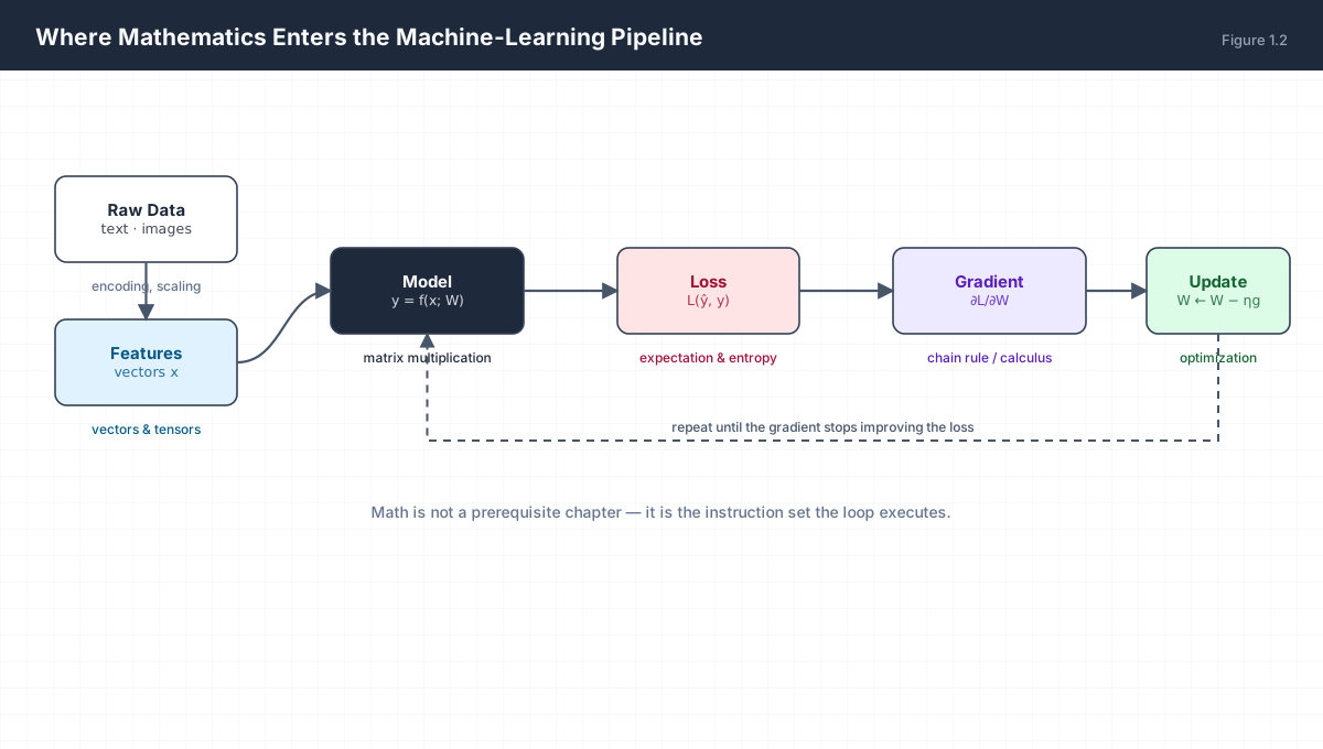
A common misconception holds that mathematics is a prerequisite to be cleared before “real” machine learning begins. The opposite is true. Mathematics is not a gate in front of the pipeline — it is the instruction set that the pipeline executes at every iteration.
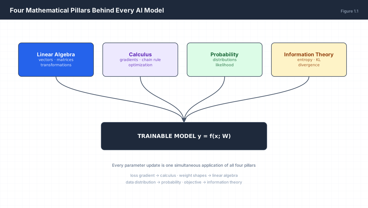
Consider the smallest possible training step. You hold a weight matrix W, you compute a prediction ŷ = f(x; W), you measure a loss L(ŷ, y), and you subtract a scaled gradient. Four distinct branches of mathematics appear in that one sentence:
| Operation in the Loop | Mathematical Branch | Symbol You Will See |
|---|---|---|
| Building a prediction | Linear algebra | y = Wx + b, W ∈ ℝ^(d_out × d_in) |
| Measuring error | Information theory / probability | L = −Σ yᵢ log ŷᵢ |
| Attributing blame | Calculus | ∂L/∂W |
| Updating parameters | Optimization (applied calculus) | W ← W − η·∂L/∂W |
| Judging generalisation | Probability / statistics | E[L] over p(x, y) |
3. Sets: The Ground Layer of Everything
A set is an unordered collection of distinct objects, called elements. If x is an element of A we write x ∈ A; if not, x ∉ A. A set with no elements is the empty set, written ∅.
Sets matter because every object in machine learning is defined as a member of one. The domain of a function is a set. The set of all possible parameter values is a set. The training dataset is a finite set of pairs. A class label space is a finite set. Even the output of a classifier is an element of a probability simplex — a specific geometric set.
3.1 Set specification methods
# Roster method: list the elements explicitly
labels = {"cat", "dog", "horse"}

# Set-builder (comprehension) method: state the rule
# B = { x ∈ ℝ | 0 ≤ x ≤ 1 }   "all reals between 0 and 1 inclusive"
unit_interval_rule = lambda x: 0.0 <= x <= 1.0

# A finite dataset is a set of (input, label) pairs
# D = { (x₁,y₁), (x₂,y₂), ..., (xₙ,yₙ) }
print(len(labels))          # 3 — sets drop duplicates
3.2 The four core operations
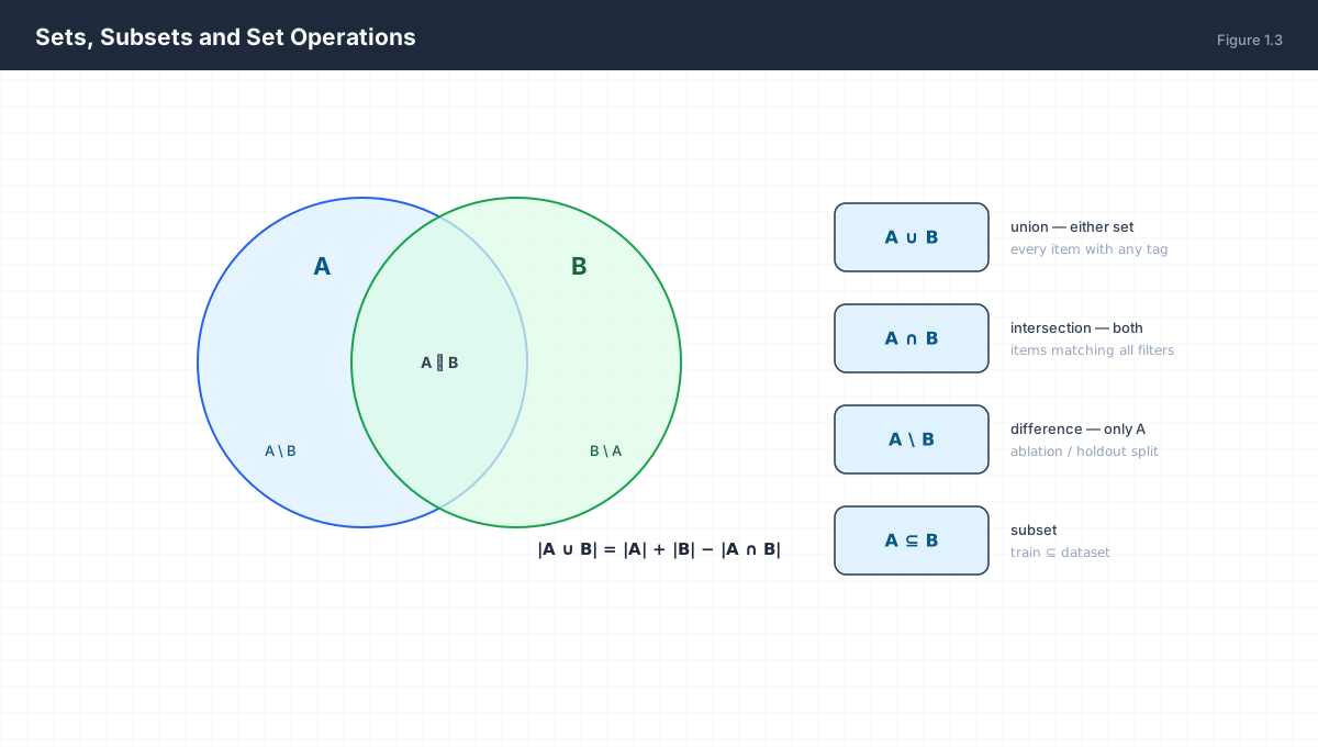
The inclusion–exclusion identity governs how cardinalities combine. It is the reason a naive "count of A plus count of B" overcounts whenever the sets overlap:
|A ∪ B| = |A| + |B| − |A ∩ B|

# Extends to three sets:
|A ∪ B ∪ C| = |A| + |B| + |C|
             − |A ∩ B| − |A ∩ C| − |B ∩ C|
             + |A ∩ B ∩ C|
This identity is not academic. If you deduplicate a corpus by computing len(set_a | set_b), you are applying inclusion–exclusion in one line — and if you instead wrote len(set_a) + len(set_b), you would overcount precisely by |A ∩ B|, silently inflating your training set and biasing every downstream evaluation metric.
3.3 Sets that appear constantly in practice
- Sample space
Ω— every outcome a random experiment could produce. The denominator of all probability. - Parameter space
Θ— every weight configuration the model could occupy. Training is a walk through this set. - Support — the set of inputs where a distribution is non-zero. A softmax over
kclasses has support of sizek. - Subset
A ⊆ B— a training split is a subset of the full dataset; the test split must be a disjoint subset.
4. Tuples, Relations and Cartesian Products
A tuple is an ordered collection. This is the crucial difference from a set: (1, 2) ≠ (2, 1), whereas {1, 2} = {2, 1}. Machine-learning data is almost always tuple-valued, because feature order carries meaning — swapping two columns of a feature matrix changes the model.
The Cartesian product A × B is the set of all ordered pairs with the first element from A and the second from B:
A = {1, 2},  B = {a, b}
A × B = {(1,a), (1,b), (2,a), (2,b)}       |A × B| = |A| · |B|
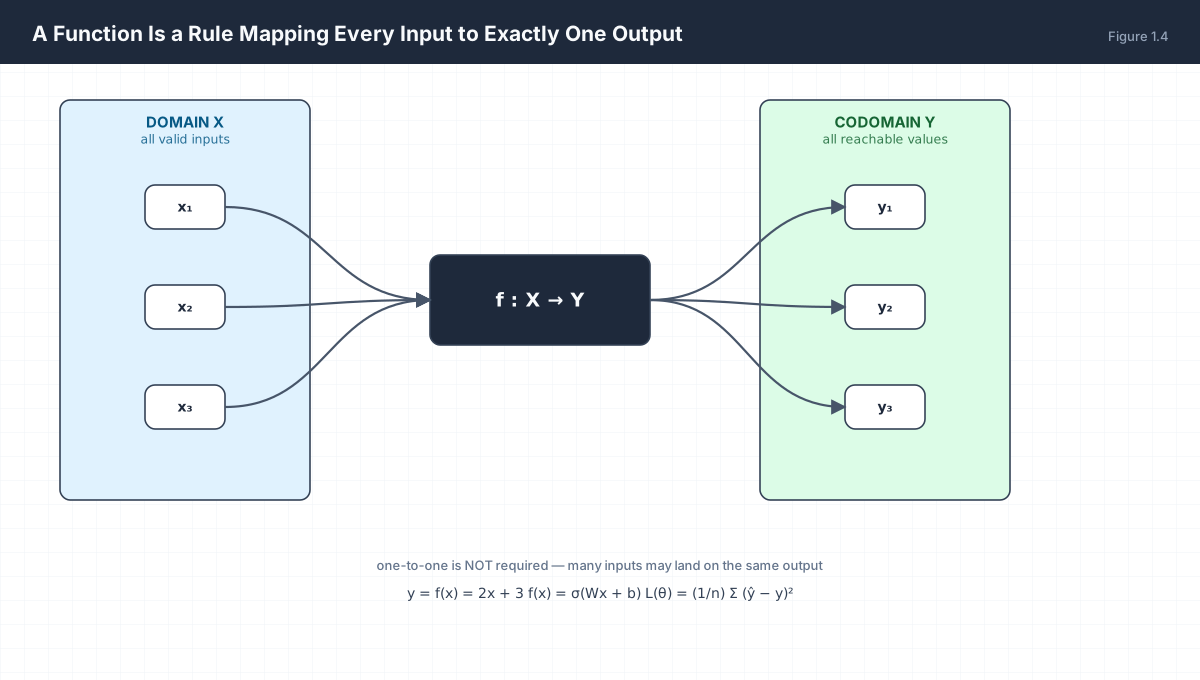
A relation from A to B is any subset of A × B. A function is a relation with an extra constraint: every element of A appears in exactly one pair. That single constraint is the entire distinction between a relation and a function, and it is what makes functions computable — given an input, there is never ambiguity about which output to return.
| Concept | Ordered? | Duplicates? | Function Constraint |
|---|---|---|---|
| Set | No | Dropped | — |
| Tuple | Yes | Allowed | — |
| Relation | Yes | Not applicable | None |
| Function | Yes | Not applicable | Exactly one output per input |
5. Functions: Domain, Codomain, Image and Composition
A function f : X → Y assigns to every element of the domain X exactly one element of the codomain Y. The set of values actually produced is the image (or range), which may be a proper subset of the codomain.
5.1 The three properties that matter
| Property | Meaning | Consequence for AI |
|---|---|---|
| Injective (one-to-one) | Distinct inputs give distinct outputs | Information is preserved; an inverse can exist on the image. |
| Surjective (onto) | Every codomain element is hit | Decoder can reach every output pattern; generative coverage. |
| Bijective | Both of the above | Invertible — the basis of normalising flows and reversible layers. |
5.2 Composition is the shape of a neural network
Given g : X → Y and f : Y → Z, the composition (f ∘ g)(x) = f(g(x)) applies g first. A four-layer network is nothing more than a four-fold composition:
# A network is function composition, written left-to-right in code
# but right-to-left in mathematical notation.
#
#   ŷ = f₄( f₃( f₂( f₁(x) ) ) )   ==   (f₄ ∘ f₃ ∘ f₂ ∘ f₁)(x)

import numpy as np

W1 = np.random.randn(784, 256) * 0.01; b1 = np.zeros(256)
W2 = np.random.randn(256, 128) * 0.01; b2 = np.zeros(128)
W3 = np.random.randn(128, 64)  * 0.01; b3 = np.zeros(64)
W4 = np.random.randn(64, 10)   * 0.01; b4 = np.zeros(10)
x  = np.random.randn(784)

def relu(h):
    return np.maximum(0.0, h)

def softmax(h):
    e = np.exp(h - h.max(axis=-1, keepdims=True))
    return e / e.sum(axis=-1, keepdims=True)

def layer1(x): return x @ W1 + b1       # affine
def layer2(h): return relu(h @ W2 + b2) # affine + nonlinearity
def layer3(h): return relu(h @ W3 + b3)
def layer4(h): return softmax(h @ W4 + b4)

y_hat = layer4(layer3(layer2(layer1(x))))
print(y_hat.shape, y_hat.sum().round(6))   # (10,) 1.0
This is the reason the chain rule (Chapter 21) is the single most important theorem in deep learning. Differentiating a composition requires differentiating each factor in order and multiplying. Backpropagation is the chain rule applied to the composition graph, computed from the output backwards.
5.3 Inverse functions and why most layers are not invertible
An inverse f⁻¹ exists only when f is bijective. ReLU — max(0, x) — is not injective, because every negative input maps to 0. That single fact is why a standard network cannot be run backwards to recover its input, and why architectures that do need reversibility (normalising flows, invertible residual networks) replace ReLU with strictly monotonic activations.
6. The Notation Ladder: Scalars, Vectors, Matrices, Tensors
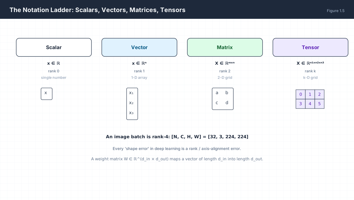
Rank is the number of axes an array possesses. It is the single most useful fact you can attach to a symbol, because almost every runtime error in deep learning is a rank or axis-alignment error wearing a different costume.
| Rung | Typographic Convention | Example in a Model |
|---|---|---|
| Rank 0 — scalar | lowercase italic x |
learning rate η, a single loss value |
| Rank 1 — vector | bold lowercase x |
one embedding, one feature row, one bias vector |
| Rank 2 — matrix | bold uppercase W |
a weight matrix, a batch of feature rows |
| Rank 3+ — tensor | calligraphic 𝒳 or bold uppercase |
attention scores, a batch of images |
A shape declaration should always be read outward from the operation. In y = Wx with W ∈ ℝ^(4×3) and x ∈ ℝ³, the inner dimensions must agree (3 = 3) and the result inherits the outer ones, giving y ∈ ℝ⁴. In the batched form Y = XW^T with X ∈ ℝ^(B×3), the batch dimension B passes through untouched: Y ∈ ℝ^(B×4).
# Reading shapes outward from the operation
# y = W x      W:(4,3)  x:(3,)      -> y:(4,)        inner dims agree
# Y = X Wᵀ     X:(B,3)  W:(4,3)     -> Y:(B,4)       batch dim preserved
# scores = Q Kᵀ / √d    Q:(B,H,T,d) K:(B,H,T,d) -> (B,H,T,T)

import numpy as np

W = np.zeros((4, 3));  x = np.zeros((3,))
X = np.zeros((8, 3))

assert W.shape[1] == x.shape[0], "inner dimensions must agree"
Y = X @ W.T
assert Y.shape == (8, 4), "batch dimension must be preserved"
print("y:", (W @ x).shape, "Y:", Y.shape)
7. Summation, Product and Index Notation
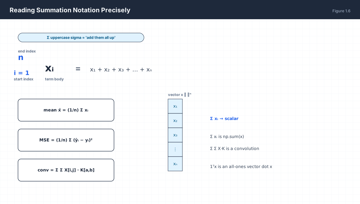
Summation notation is the compression scheme that turns a loop into a single expression. Every Σ you meet in a paper has exactly one honest translation into array code, and learning that translation is worth more than memorising a hundred formulas.
7.1 The three symbols you need
| Symbol | Name | Meaning |
|---|---|---|
| Σ | Sigma | Add the terms: Σᵢ₌₁ⁿ xᵢ = x₁ + … + xₙ |
| Π | Pi | Multiply the terms: Πᵢ₌₁ⁿ pᵢ — the joint probability of independent events |
| ∫ | Integral | Continuous summation — expectation over a density |
7.2 Nested sums and their array equivalents
import numpy as np

A = np.array([[1., 2.], [3., 4.]])
B = np.array([[5., 6.], [7., 8.]])

# Σᵢ Σⱼ A[i,j]              -> one scalar: total of every element
total = A.sum()

# Σⱼ A[i,j]                 -> per-row sum, collapses axis 1, result shape (2,)
row_sums = A.sum(axis=1)

# Σᵢ A[i,j]                 -> per-column sum, collapses axis 0, result shape (2,)
col_sums = A.sum(axis=0)

# Σⱼ A[i,j] · B[j,k]        -> matrix product, shape (2,2)
matmul = A @ B

# Σᵢ A[i,j] · B[i,j]        -> elementwise product then total: the Frobenius inner product
frob = (A * B).sum()

print(total, row_sums, col_sums, frob)
# 10.0 [3. 7.] [4. 6.] 70.0
Two rules make nested sums decodable. First, each summation sign removes exactly one axis, so the number of Σs tells you the rank drop. Second, the order of summation does not matter for a finite sum — you may evaluate whichever index is cheapest first, which is precisely the freedom that lets a compiler reorder reductions and lets you choose between einsum, matmul, or a broadcasted multiply.
7.3 Einstein summation
Einstein notation drops the Σ entirely by the convention that any index appearing twice in a term is summed over. It is the native language of tensor libraries:
import numpy as np

A = np.random.rand(2, 3)
B = np.random.rand(3, 4)

# Σⱼ A[i,j] · B[j,k]   is written   A_ij B_jk   in Einstein notation
result = np.einsum('ij,jk->ik', A, B)   # identical to A @ B

# Batched attention scores: Σ_d Q[b,h,i,d] · K[b,h,j,d]
B, H, T, d = 2, 4, 8, 16
Q = np.random.rand(B, H, T, d)
K = np.random.rand(B, H, T, d)
scores = np.einsum('bhid,bhjd->bhij', Q, K)
print(scores.shape)   # (2, 4, 8, 8)
8. Greek Symbols and Paper Conventions
Research papers use Greek letters with remarkable consistency. Learning the conventional mappings removes most of the friction from reading them.
| Symbol | Name | Standard Meaning |
|---|---|---|
| θ | theta | All trainable parameters, taken as one vector |
| η | eta | Learning rate |
| λ | lambda | Regularisation strength; also an eigenvalue |
| σ | sigma | Sigmoid; standard deviation; singular value |
| μ | mu | Mean of a distribution |
| ∇ | nabla | Gradient operator — vector of partial derivatives |
| ε | epsilon | Small constant for numerical stability; also noise |
| ∂ | partial | Partial derivative, holding other variables fixed |
8.1 Decorative notation that carries real information
- Hat
ŷ— a prediction or estimate, as opposed to the observed truthy. - Bar
x̄— the arithmetic mean of a collection. - Subscript
xᵢ— the i-th element of a collection; not "x times i". - Superscript
x⁽ˡ⁾— the value at layer l. Beware: this is not exponentiation. Context disambiguates, and layer superscripts are almost always parenthesised. - T
Wᵀ— transpose: axes swapped. ForW ∈ ℝ^(m×n),Wᵀ ∈ ℝ^(n×m).
9. Reading a Model Equation Aloud
The test of notation literacy is whether you can narrate an equation. Take the workhorse of the field:
ŷ = softmax(W x + b)

"y-hat equals softmax of W times x plus b"

ŷ        the predicted probability vector over classes
W        a weight matrix of shape (n_classes, n_features)
x        the input feature vector of shape (n_features,)
W x      a matrix-vector product: mixes every feature into every class score
b        a bias vector of shape (n_classes,), one offset per class
W x + b  the affine map — a linear transform followed by a translation
softmax  normalises the raw scores into a probability distribution
And its batched, deep counterpart — the form most papers actually write:
H⁽ˡ⁺¹⁾ = σ( H⁽ˡ⁾ Wᵀ⁽ˡ⁾ + b⁽ˡ⁾ )

H⁽ˡ⁾     activations at layer l, shape (B, d_l)   — B is the batch dimension
W⁽ˡ⁾     weight matrix of layer l, shape (d_{l+1}, d_l)
σ        an elementwise nonlinearity applied independently to each entry
H⁽ˡ⁺¹⁾   activations at layer l+1, shape (B, d_{l+1})
Note that σ is applied elementwise, so it never changes shape. Only the matrix product changes shape, and it changes exactly one axis — the feature axis. The batch axis passes through the entire network untouched. That single observation eliminates the majority of shape bugs in practice.
10. Worked Examples
10.1 Set cardinality with overlap
A training set has 4,800 reviews. 3,200 are positive, 2,100 are negative, and 500 are labelled both (multi-label sentiment). How many distinct reviews exist?
|P ∪ N| = |P| + |N| − |P ∩ N| = 3200 + 2100 − 500 = 4800 ✓
The identity is consistent with the stated total. If the union had come out below 4,800, the labels would contain duplicates; above, some reviews would be unlabelled.
10.2 Determining whether a relation is a function
Given R = {(1,2), (2,4), (3,6), (1,8)} on {1,2,3} → {2,4,6,8}: is R a function?
No. The input 1 appears twice, mapped to 2 and to 8. A function requires exactly one output per input. Removing either pair makes it a function; this is precisely the constraint a database primary key enforces.
10.3 Composing three layers and tracking shape
Let x ∈ ℝ^(784), W₁ ∈ ℝ^(256×784), W₂ ∈ ℝ^(10×256). Compute the output shape.
h  = σ(W₁x)     (256×784)·(784)  -> (256)
ŷ  = softmax(W₂h) (10×256)·(256) -> (10)
784 → 256 → 10        two matrix products, two axis changes, no others.
10.4 Evaluating a nested sum by hand
Compute Σᵢ₌₁² Σⱼ₌₁³ (i + j).
i=1:  (1+1)+(1+2)+(1+3) = 2+3+4 = 9
i=2:  (2+1)+(2+2)+(2+3) = 3+4+5 = 12
total = 9 + 12 = 21
Two summation signs, and the result is rank 0 — a scalar. Each Σ removed one axis.
10.5 Rescaling a loss by the summation formulation
Express mean squared error over n samples as a summation, then as an array reduction.
MSE = (1/n) Σᵢ₌₁ⁿ (ŷᵢ − yᵢ)²

Python:  ((y_hat - y) ** 2).mean()
NumPy:   np.mean((y_hat - y) ** 2)
The 1/n outside the sum is what converts a total into an average. Move it inside and you have a per-sample loss vector instead of a scalar — a distinction that matters the moment you introduce sample weighting.
11. Verify It in Python
Every claim in this chapter is checkable in a few lines. Run this to confirm the identities rather than trusting them.
import numpy as np

# --- 1. Inclusion–exclusion identity -------------------------------
A = {f"review_{i}" for i in range(3200)}          # 3200 elements
B = {f"review_{i}" for i in range(2700, 4800)}     # 2100 elements, 500 overlap
lhs = len(A | B)
rhs = len(A) + len(B) - len(A & B)
assert lhs == rhs, (lhs, rhs)
print(f"union={lhs}  identity={rhs}  overlap={len(A & B)}")

# --- 2. A function has exactly one output per input -----------------
R = [(1, 2), (2, 4), (3, 6)]
is_function = len({a for a, _ in R}) == len(R)
print("is_function:", is_function)          # True

# --- 3. Shape propagation through a stack --------------------------
x  = np.random.randn(784)
W1 = np.random.randn(256, 784)
W2 = np.random.randn(10, 256)

h = np.maximum(0.0, W1 @ x)                 # (256,)
y = W2 @ h                                  # (10,)
assert h.shape == (256,) and y.shape == (10,)
print("shapes:", h.shape, y.shape)

# --- 4. Nested summation, both signs -------------------------------
manual = sum((i + j) for i in range(1, 3) for j in range(1, 4))
assert manual == 21
print("nested sum:", manual)

# --- 5. Sigmoid numerics: why epsilon exists -----------------------
def naive_sigmoid(z):
    return 1.0 / (1.0 + np.exp(-z))

for z in (-800.0, 800.0):
    with np.errstate(over="raise"):
        try:
            print(z, naive_sigmoid(np.float64(z)))
        except FloatingPointError:
            print(z, "FloatingPointError: np.exp overflowed to inf")
The final block is the first practical reason for the stability constants met throughout this series. For sufficiently negative z, np.exp(-z) overflows to infinity and the division underflows to zero — silently, in most vectorised code. Chapter 47 returns to this problem with the numerically stable formulation.
12. Practice Questions
- Let
A = {1, 2, 3, 4}andB = {3, 4, 5}. ComputeA ∪ B,A ∩ B,A \ B, andA × B, and state the cardinality of each. - Why is the relation
{(a,1), (b,2), (c,2)}a valid function while{(a,1), (a,2)}is not, even though both are subsets of a Cartesian product? - A layer maps
ℝ^(512) → ℝ^(128). State the exact shape of its weight matrix and bias vector, then give the batched shapes for a batch ofB = 32. - Translate
Σᵢ₌₁ⁿ Σⱼ₌₁ᵐ C[i,j]into NumPy, then translateΣₖ A[i,k] B[k,j]and name the operation. - Explain why applying an activation function elementwise can never change a tensor's shape, while a matrix product always can.
- Given that
ReLUis not injective, describe one architectural workaround that restores invertibility for a reversible network. - Expand
Πᵢ₌₁³ (1 − pᵢ)and interpret it probabilistically for three independent events. - In
H⁽ˡ⁺¹⁾ = σ(H⁽ˡ⁾Wᵀ⁽ˡ⁾ + b⁽ˡ⁾), which symbol encodes the layer index and how do you know it is not an exponent? - You observe
Y ∈ ℝ^(32×768×128)after a projection fromX ∈ ℝ^(32×768×64). Which axis changed, and what shape was the weight matrix? - Why does the inclusion–exclusion identity matter when deduplicating a training corpus, and what specific metric gets biased if it is ignored?
13. Official References & Further Reading
- Goodfellow, Bengio & Courville — Deep Learning, Part I: Applied Math and Machine Learning Basics
- Deisenroth, Faisal & Ong — Mathematics for Machine Learning (free PDF)
- NumPy —
einsumReference and Einstein Summation Convention - 3Blue1Brown — Essence of Linear Algebra (visual series)
- Set Theory — Elements, Subsets and Set Operations
Continue the Course
- Course Index: AI Mathematics Masterclass — All 48 Chapters
- Next Chapter: Chapter 2: Linear Equations, Systems & Solving for Unknowns
- Related Series: PyTorch Engineering Masterclass — All 16 Modules