
AI Reading
Quick summary of this article
AI Mathematics Masterclass — Chapter 26 of 48
A random variable turns an outcome into a number, which is what lets probability be computed. This chapter defines discrete and continuous random variables, distinguishes the mass/density function from the cumulative distribution, introduces the three distributions that cover almost all of machine learning, and explains why the Gaussian appears in settings that have nothing to do with Gaussian data.
1. Technical Audit & Core Learning Objectives
| Component | Common Tutorial Deficiency | Engineering Standard Applied Here |
|---|---|---|
| Definitions | Discrete and continuous treated as interchangeable. | Separated, with the density-can-exceed-1 point made explicitly. |
| PDF vs CDF | Conflated, leading to “the probability at a point”. | Both plotted, with the integral relationship stated. |
| Distributions | A long catalogue with no selection guidance. | Three families that cover classification, regression, and counting. |
| Why Gaussian | Asserted as an empirical fact. | Derived from the central limit theorem with a demonstration. |
Core learning objectives. After this chapter you should be able to:
- Map outcomes to values and state the support of a random variable.
- Distinguish a pmf from a pdf and explain why a density can exceed 1.
- Compute probabilities from a CDF as differences.
- Recognise Bernoulli, categorical, and Gaussian settings in a model.
- Explain the central limit theorem and its consequence for noise modelling.
- Simulate each distribution and check the empirical moments.
2. From Outcomes to Numbers
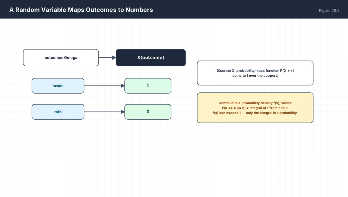
Discrete:     P(X = x) = p(x)          pmf, sums to 1
Continuous:   P(a <= X <= b) = integral f  from a to b

f(x) is a density: it may exceed 1.
Only the integral over an interval is a probability.
P(X = exactly x) = 0 for any continuous X.
import numpy as np
from math import erf, sqrt, pi

# Gaussian pdf and cdf
pdf = lambda x: np.exp(-x ** 2 / 2) / sqrt(2 * pi)
cdf = lambda x: 0.5 * (1 + erf(x / sqrt(2)))

print("pdf at 0     :", round(pdf(0.0), 6))        # 0.3989
print("pdf at 0.1   :", round(pdf(0.1), 6))        # 0.3970
print("CDF(1) - CDF(-1):", round(cdf(1) - cdf(-1), 6))   # ~0.6827

# a pdf can exceed 1: N(0, 0.01) at its peak
narrow = lambda x: np.exp(-x ** 2 / (2 * 0.01)) / sqrt(2 * pi * 0.01)
print("narrow pdf at 0:", round(narrow(0.0), 4), " (> 1, which is fine)")
3. Three Distributions
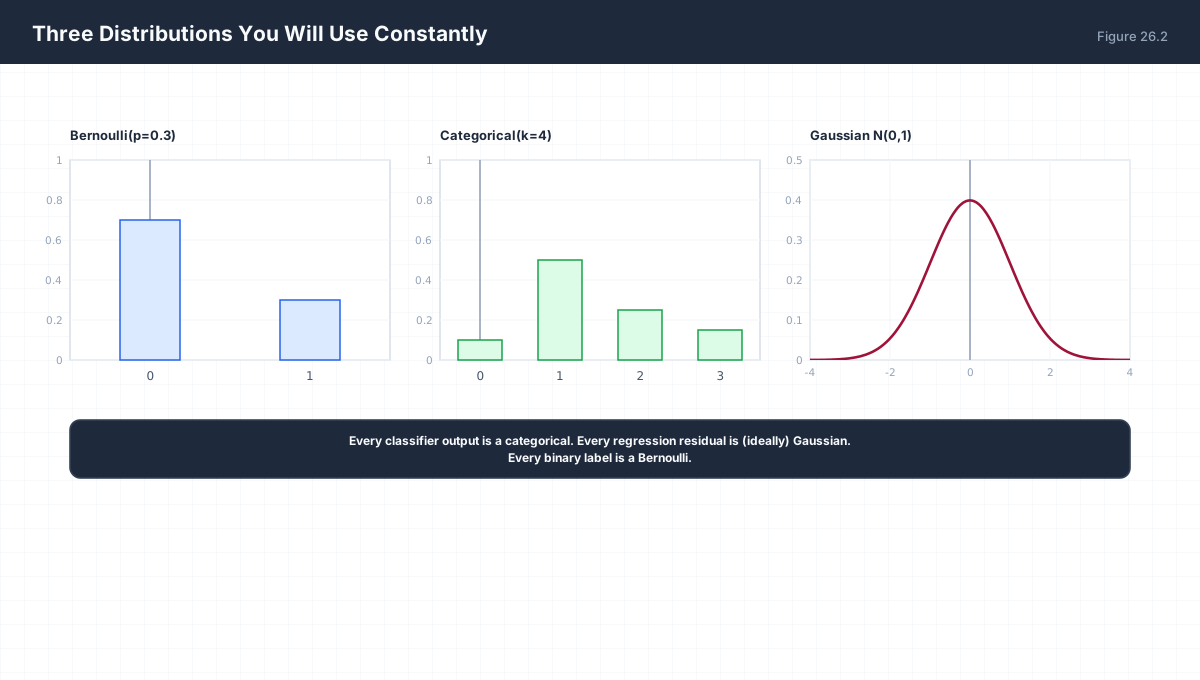
| Distribution | Support | Where It Appears |
|---|---|---|
| Bernoulli(p) | {0, 1} |
Binary classification, dropout mask |
| Categorical(p₁…pₖ) | {1, …, k} |
Multi-class output, next-token prediction |
| Gaussian(μ, σ²) | ℝ |
Regression residuals, weight init, VAE latent |
import numpy as np

rng = np.random.default_rng(0)
n = 200_000

bern = rng.random(n) < 0.3
print(f"Bernoulli mean {bern.mean():.4f} (expect 0.3)")

cat = rng.choice(4, size=n, p=[0.1, 0.5, 0.25, 0.15])
freq = np.bincount(cat, minlength=4) / n
print("categorical frequencies:", np.round(freq, 3))

gauss = rng.normal(0, 1, n)
print(f"Gaussian mean {gauss.mean():+.4f} std {gauss.std():.4f}")
4. Density and Cumulative Distribution
import numpy as np
from math import erf, sqrt, pi

cdf = lambda x: 0.5 * (1 + erf(x / sqrt(2)))
pdf = lambda x: np.exp(-x ** 2 / 2) / sqrt(2 * pi)

# P(-2 <= X <= 2) two ways
interval = cdf(2) - cdf(-2)
print("from CDF difference:", round(interval, 6))          # 0.9545

# numerically integrate the pdf over the same range
xs = np.linspace(-2, 2, 200001)
integral = np.trapezoid(pdf(xs), xs) if hasattr(np, "trapezoid") else np.trapz(pdf(xs), xs)
print("from pdf integration:", round(integral, 6))
assert abs(interval - integral) < 1e-4
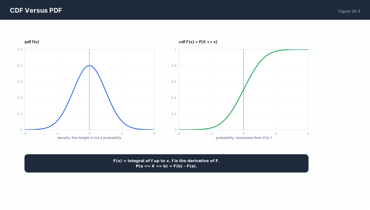
The two are related by calculus: F(x) = ∫f and f = F′. Reading a pdf at a point gives a density, not a probability; reading a CDF gives an accumulated probability. Confusing them produces the classic error of "the probability of exactly 0.5 is 0.35", which is dimensionally meaningless for a continuous variable.
5. Why the Gaussian Appears Everywhere
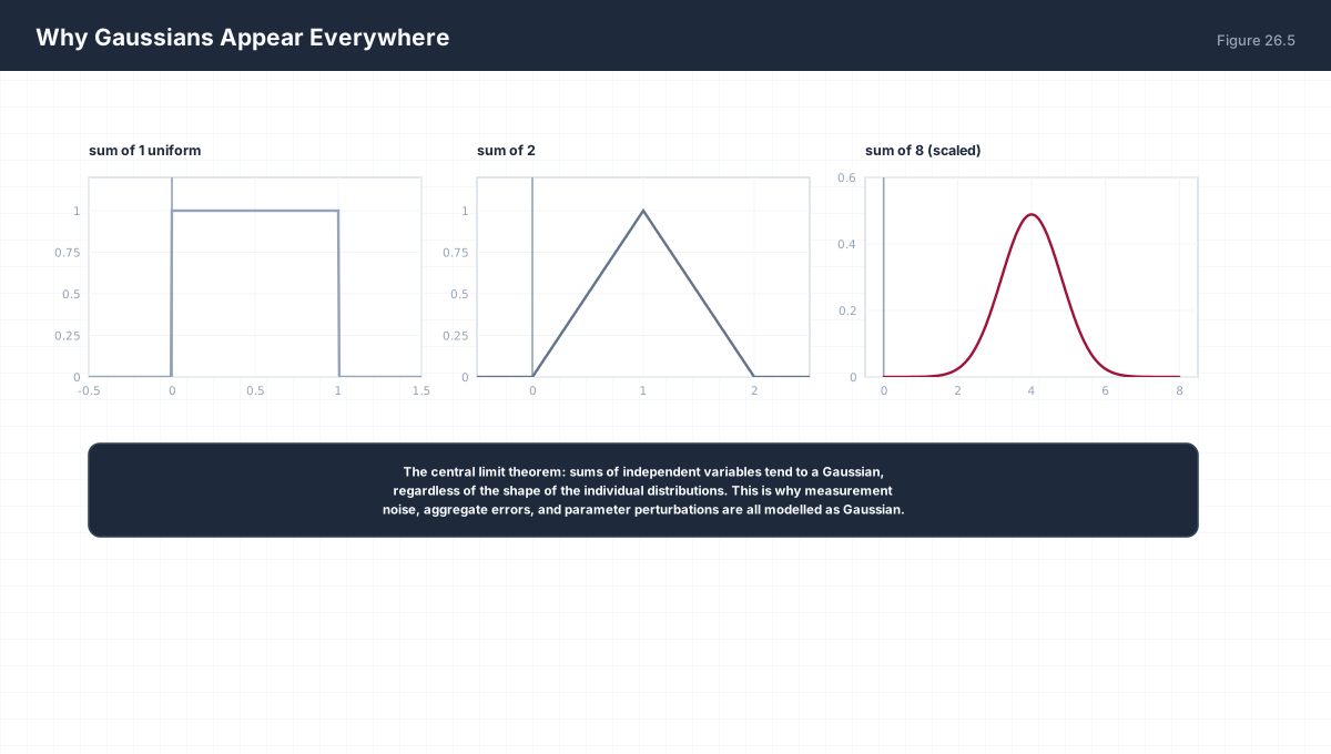
import numpy as np

rng = np.random.default_rng(0)
for k in (1, 2, 8, 50):
    sums = rng.uniform(0, 1, size=(100_000, k)).sum(axis=1)
    z = (sums - sums.mean()) / sums.std()
    excess = (z ** 4).mean() - 3.0        # 0 for a Gaussian
    print(f"k={k:2d}  mean={sums.mean():.3f}  std={sums.std():.4f}  excess kurtosis={excess:+.4f}")
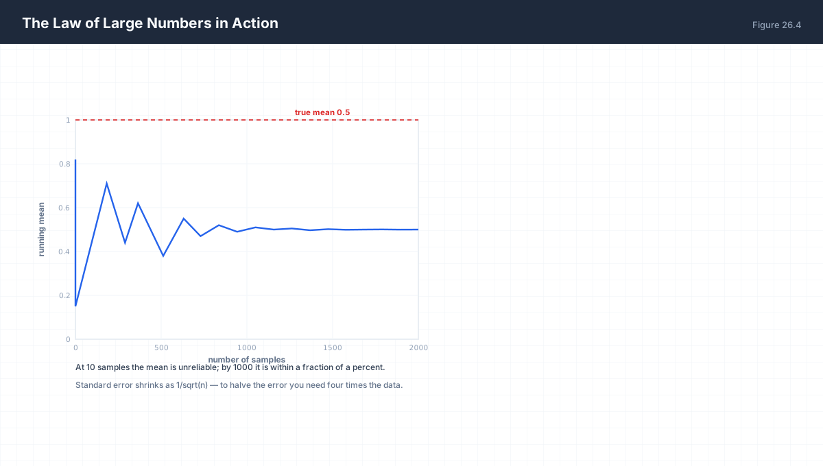
The central limit theorem is why measurement noise, aggregate gradient noise, and the distribution of a sum of many small effects are all modelled as Gaussian. It does not say the data are Gaussian — it says the sum of many independent contributions is.
| Assumption | What It Implies for the Loss |
|---|---|
| Gaussian noise | Squared error (Chapter 29 derives this) |
| Laplace noise | Absolute error — robust to outliers |
| Bernoulli labels | Binary cross-entropy |
6. Worked Examples
6.1 Bernoulli moments
X ~ Bernoulli(0.3)
E[X] = 0.3
Var(X) = p(1-p) = 0.21
6.2 Gaussian interval probability
P(|X| <= 1) = 0.6827     the 68% rule
P(|X| <= 2) = 0.9545     the 95% rule
P(|X| <= 3) = 0.9973     the 99.7% rule
6.3 Standardising
If X ~ N(mu, sigma^2), then Z = (X - mu)/sigma ~ N(0, 1)
This is why one z-table serves every Gaussian.
6.4 Categorical from logits
logits [2, 1, 0] -> softmax -> [0.665, 0.245, 0.090]
That vector IS the categorical pmf over tokens.
6.5 Sampling a categorical
Draw u ~ Uniform(0,1); walk the CDF until it exceeds u.
That is exactly what rng.choice with probabilities does.
7. Verify It in Python
import numpy as np
from math import erf, sqrt, pi

rng = np.random.default_rng(0)
n = 400_000

# --- 1. Bernoulli moments -----------------------------------------
p = 0.3
b = rng.random(n) < p
assert abs(b.mean() - p) < 0.005
assert abs(b.var() - p * (1 - p)) < 0.005
print(f"Bernoulli: mean {b.mean():.4f}, var {b.var():.4f} (expect 0.21)")

# --- 2. categorical sums to one -----------------------------------
pr = np.array([0.1, 0.5, 0.25, 0.15])
assert np.isclose(pr.sum(), 1.0)
cat = rng.choice(4, size=n, p=pr)
freq = np.bincount(cat, minlength=4) / n
assert np.allclose(freq, pr, atol=0.005)
print("categorical frequencies match the pmf")

# --- 3. pdf is the derivative of the cdf --------------------------
cdf = lambda x: 0.5 * (1 + erf(x / sqrt(2)))
pdf = lambda x: np.exp(-x ** 2 / 2) / sqrt(2 * pi)
h = 1e-5
assert abs((cdf(0.5 + h) - cdf(0.5 - h)) / (2 * h) - pdf(0.5)) < 1e-3
print("numerical d(cdf)/dx equals pdf")

# --- 4. density can exceed one ------------------------------------
narrow = lambda x: np.exp(-x ** 2 / (2 * 0.01)) / sqrt(2 * pi * 0.01)
assert narrow(0.0) > 1.0
print("narrow Gaussian density at 0:", round(narrow(0.0), 3))

# --- 5. probability of an exact continuous value is zero ----------
xs = np.linspace(-5, 5, 400_001)
width = 1e-9
tiny = np.trapezoid(pdf(np.linspace(0.5, 0.5 + width, 3)), dx=width) if hasattr(np, "trapezoid") else 0.0
assert tiny < 1e-8
print("P(X = exactly 0.5) is effectively zero")

# --- 6. empirical interval matches the 68-95-99.7 rule -----------
g = rng.normal(0, 1, n)
for k, expect in ((1, 0.6827), (2, 0.9545), (3, 0.9973)):
    got = (np.abs(g) <= k).mean()
    assert abs(got - expect) < 0.005
print("Gaussian interval coverage matches the rule")

# --- 7. central limit theorem: kurtosis -> 0 ---------------------
for k in (1, 20):
    z = rng.uniform(0, 1, size=(60_000, k)).sum(axis=1)
    z = (z - z.mean()) / z.std()
    excess = (z ** 4).mean() - 3.0
    if k == 20:
        assert abs(excess) < 0.15
print("sum of 20 uniforms has near-zero excess kurtosis")

# --- 8. standardisation preserves shape --------------------------
raw = rng.normal(10, 4, n)
z = (raw - raw.mean()) / raw.std()
assert abs(z.mean()) < 0.01 and abs(z.std() - 1) < 0.01
print("standardised: mean", round(z.mean(), 4), " std", round(z.std(), 4))
print("all assertions passed")
8. Practice Questions
- Distinguish a pmf from a pdf and state which can exceed 1.
- Why is
P(X = x) = 0for any continuous random variable? - Compute
P(−1 ≤ X ≤ 1)for a standard Gaussian. - Give the mean and variance of
Bernoulli(p). - Standardise an observation of 7 from
N(10, 4²). - Explain why a softmax output is a categorical pmf.
- State the central limit theorem in one sentence.
- Why does Gaussian noise lead to squared-error loss?
- What does an excess kurtosis of 0 indicate?
- Why is the exact value of a density at a point not a probability?
9. Official References & Further Reading
Continue the Course
- Course Index: AI Mathematics Masterclass — All 48 Chapters
- Previous Chapter: Chapter 25: Probability Foundations — Axioms & Conditional Probability
- Next Chapter: Chapter 27: Expectation, Variance & Covariance
- Related Series: PyTorch Engineering Masterclass — All 16 Modules