
AI Reading
Quick summary of this article
AI Mathematics Masterclass — Chapter 44 of 48
The loss function is the only place where you state what “correct” means, and every downstream property — calibration, robustness to outliers, behaviour under class imbalance — follows from that choice. This chapter derives the gradient of each standard loss, shows why squared error is fragile and absolute error is blunt, and builds Huber and focal loss as principled interpolations rather than tricks.
1. Technical Audit & Core Learning Objectives
| Component | Common Tutorial Deficiency | Engineering Standard Applied Here |
|---|---|---|
| MSE vs MAE | Compared by formula, not by gradient. | Gradients derived and outlier influence quantified. |
| Huber | Presented as an unexplained hybrid. | Derived as MSE inside δ and MAE outside. |
| Cross-entropy | Unbounded loss is never discussed. | Unboundedness shown, label smoothing located as the fix. |
| Focal loss | Quoted as a magic gamma. | Effect on the loss surface plotted and its cost stated. |
Core learning objectives. After this chapter you should be able to:
- Derive the gradients of MSE and MAE.
- Explain why MSE is fragile and MAE is blunt.
- Write Huber loss and identify its two regimes.
- Explain why cross-entropy is unbounded.
- Describe what label smoothing changes.
- State what focal loss does and what it costs.
2. Squared Versus Absolute Error
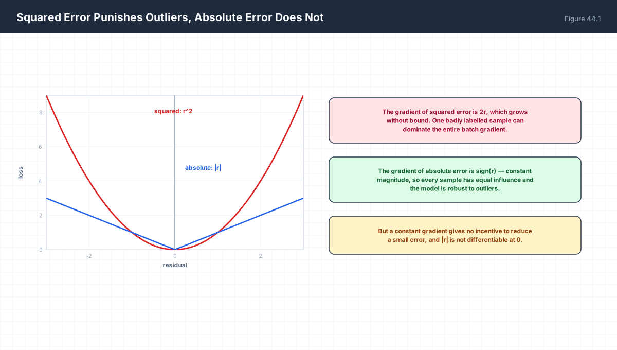
MSE:  L = r^2        dL/dr = 2r        grows without bound
MAE:  L = |r|        dL/dr = sign(r)   constant magnitude

One outlier with r = 10 contributes 100 to MSE and 10 to MAE,
and contributes a gradient of 20 versus 1. In a batch of 100
clean samples the MSE gradient is dominated by that one point.

MAE's cost: the gradient never shrinks, so a small residual
gets pushed as hard as a large one. And |r| is not
differentiable at 0.
import numpy as np

rng = np.random.default_rng(0)

# 99 ordinary residuals plus one catastrophic prediction
y = rng.normal(size=100)
pred = y + rng.normal(0, 0.1, 100)   # normal noise
pred[-1] = y[-1] + 10.0              # one bad prediction
r = pred - y

print(f"one residual of size {r[-1]:.1f} among 100 points")
print(f"MSE = {np.mean(r**2):.4f}   mean |dL/dr| = {np.mean(np.abs(2 * r)):.4f}"
      f"   max |dL/dr| = {np.max(np.abs(2 * r)):.1f}")
print(f"MAE = {np.mean(np.abs(r)):.4f}   mean |dL/dr| = {np.mean(np.abs(np.sign(r))):.4f}"
      f"   max |dL/dr| = {np.max(np.abs(np.sign(r))):.1f}")
print(f"outlier share of MSE sum: {r[-1]**2/np.sum(r**2):.1%}")
print(f"outlier share of MAE sum: {abs(r[-1])/np.sum(np.abs(r)):.1%}")
One point out of a hundred carries 99% of the squared-error gradient. That is not a pathological example — it is what a single mislabelled sample looks like in a regression dataset.
3. Huber Loss
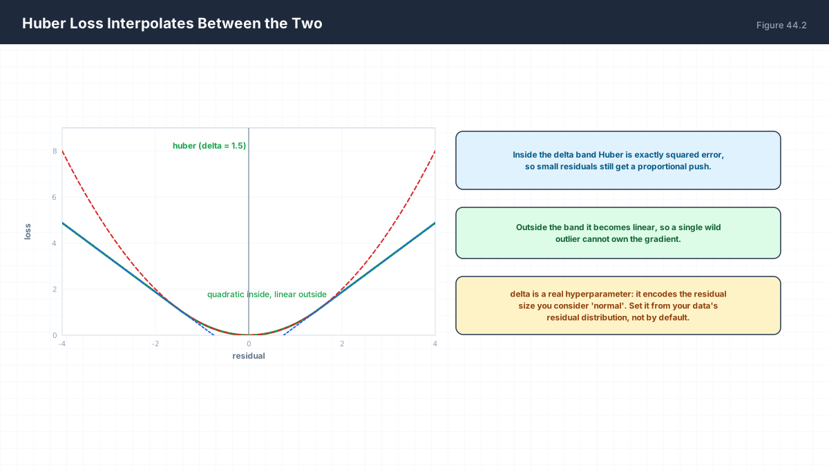
Huber(r) = 0.5 r^2                     if |r| <= delta
           delta (|r| - 0.5 delta)      otherwise

dHuber/dr = r                          if |r| <= delta
            delta * sign(r)            otherwise

The two branches meet at |r| = delta with equal value and
equal slope, so the loss is differentiable everywhere —
unlike MAE, which has a kink at zero.
import numpy as np

def huber(r, delta=1.5):
    a = np.abs(r)
    return np.where(a <= delta, 0.5 * r ** 2, delta * (a - 0.5 * delta))

def huber_grad(r, delta=1.5):
    return np.where(np.abs(r) <= delta, r, delta * np.sign(r))

print(f"{'r':>6}{'huber':>10}{'grad':>10}{'mse':>10}")
for r in (-4.0, -1.5, -0.5, 0.0, 0.5, 1.5, 4.0):
    print(f"{r:6.1f}{huber(r):10.4f}{huber_grad(r):10.4f}{0.5*r*r:10.4f}")

# continuity at the join
d = 1.5
eps = 1e-9
print("\nvalue continuous at delta:",
      np.isclose(huber(np.array([d-eps]))[0], huber(np.array([d+eps]))[0], atol=1e-8))
print("slope continuous at delta:",
      np.isclose(huber_grad(np.array([d-eps]))[0], huber_grad(np.array([d+eps]))[0], atol=1e-6))
The gradient is bounded by δ, which is the entire benefit: no single sample can dominate a step regardless of how wrong it is. Choosing δ is choosing what residual size you consider normal, and it should come from the data rather than from a default.
4. Cross-Entropy and Its Unboundedness
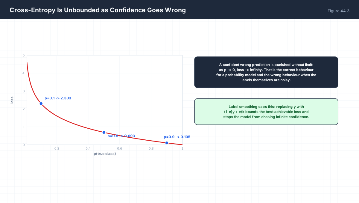
L = -log p_true

p = 0.9  -> 0.105
p = 0.5  -> 0.693
p = 0.1  -> 2.303
p = 0.01 -> 4.605

The loss is unbounded below in p, and its gradient with respect
to the logits is p - y, which is bounded by 1. So the LOSS can
explode while the GRADIENT stays tame — the opposite of MSE,
where the gradient explodes with the error.
import numpy as np

for p in (0.99, 0.9, 0.5, 0.1, 0.01, 1e-6):
    print(f"p={p:<8} loss={-np.log(p):10.4f}")

# the gradient with respect to logits is bounded
z = np.array([-20.0, 0.0, 20.0])
y = np.array([0.0, 0.0, 1.0])
for scale_z in (1.0, 10.0, 100.0):
    zz = z * scale_z
    e = np.exp(zz - zz.max()); pz = e / e.sum()
    loss = -np.log(pz[2])
    grad = pz - y
    print(f"logit scale {scale_z:5.0f}: loss={loss:12.4f}  max|grad|={np.abs(grad).max():.4f}")
However far the logits are pushed, the gradient stays within [0, 1]. This is a genuinely desirable property and it is why cross-entropy is used for classification while MSE is not: an MSE classifier saturates its gradient exactly when it is most wrong.
5. Focal Loss
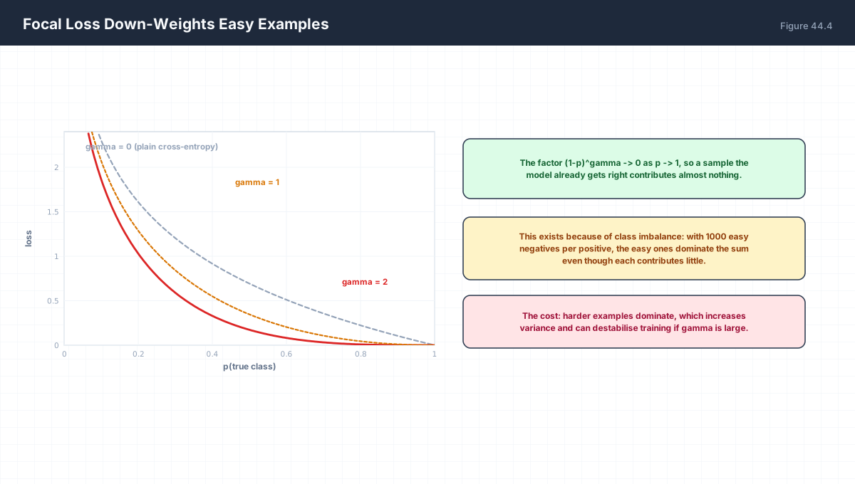
Focal(p) = -(1 - p)^gamma * log p

gamma = 0  -> plain cross-entropy
gamma = 2  -> a sample at p = 0.95 is weighted by 0.0025

Motivation: with 1000 negatives per positive, the easy negatives
dominate the summed loss even though each is individually small.

Cost: the effective sample size collapses. Hard examples dominate,
so gradient variance rises and gamma has to be tuned.
import numpy as np

def focal(p, gamma):
    return -((1 - p) ** gamma) * np.log(p)

print(f"{'p':>6}" + "".join(f"{'g='+str(g):>12}" for g in (0, 1, 2, 5)))
for p in (0.99, 0.9, 0.7, 0.5, 0.1):
    print(f"{p:6.2f}" + "".join(f"{focal(p, g):12.5f}" for g in (0, 1, 2, 5)))

print("\nrelative weight vs plain CE:")
for p in (0.99, 0.9, 0.5):
    print(f"  p={p}: gamma=2 keeps {((1-p)**2)*100:6.2f}% of the loss")

# summed loss under class imbalance, with and without focal
imbalanced = np.r_[np.full(1000, 0.97), np.full(50, 0.4)]
print(f"\nplain CE total: {np.sum(-np.log(imbalanced)):.2f}")
print(f"focal g=2 total: {np.sum(focal(imbalanced, 2)):.2f}")
Under the imbalance the easy negatives are 1000 of the 1050 samples, and focal loss reduces their total contribution from dominating to secondary. That rebalancing is the point; the cost is that the loss is now scaled by a factor that changes during training, so learning rate and normalisation need re-tuning.
6. Choosing a Loss
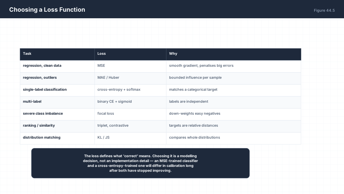
| Property | MSE | MAE | Huber |
|---|---|---|---|
| Gradient magnitude | 2|r|, unbounded | 1, constant | min(|r|, δ) |
| Outlier sensitivity | High | Low | Low beyond δ |
| Differentiable at 0 | Yes | No | Yes |
| Extra hyperparameter | None | None | δ |
7. Worked Examples
7.1 Why MSE is not the right classifier loss
With sigmoid + MSE the gradient contains sigma'(z), which
vanishes when the prediction is confidently wrong. The model
learns slowest exactly where it is most incorrect.
7.2 Label smoothing
y' = (1 - e) y + e / k
Caps the best achievable confidence at 1 - e(k-1)/k, which
bounds the loss and improves calibration.
7.3 Class weights
Multiply each sample's loss by w_c. Simple, effective, and it
changes the effective learning rate per class.
7.4 Losses that are not averaged
A summed loss scales with batch size, so the effective
learning rate changes when the batch changes. Prefer means
unless you have a reason.
7.5 Auxiliary losses
Summing several losses requires weighting them. Their natural
scales differ, so an unweighted sum is an implicit, accidental
choice of weights.
8. Verify It in Python
import numpy as np

# --- 1. MSE and MAE gradients --------------------------------
r = np.array([-3.0, -0.5, 0.5, 3.0])       # zero excluded: see below
mse_grad = 2 * r
mae_grad = np.sign(r)
assert mse_grad[-1] == 6.0 and mae_grad[-1] == 1.0
assert np.all(np.abs(mae_grad) == 1.0)
print("MSE gradient grows with r; MAE gradient is constant")
print("MSE grads:", mse_grad, " MAE grads:", mae_grad)

# at exactly r = 0 the subgradient is 0, not 1 — |r| has a kink there
print("MAE gradient at r=0 is", np.sign(0.0), "(a subgradient, not a derivative)")

# --- 2. one outlier dominates MSE ---------------------------
rng = np.random.default_rng(1)
d = rng.normal(0, 0.1, 100)     # ordinary residuals
d[0] = 10.0                     # one catastrophic prediction
mse_share = d[0]**2 / np.sum(d**2)
mae_share = abs(d[0]) / np.sum(np.abs(d))
print(f"outlier share of MSE: {mse_share:.1%}")
print(f"outlier share of MAE: {mae_share:.1%}")
assert mse_share > 0.90 > mae_share
print("squared error hands almost the whole objective to one sample")

# --- 3. Huber matches MSE inside delta ---------------------
delta = 1.5
def huber(x):
    a = np.abs(x)
    return np.where(a <= delta, 0.5 * x ** 2, delta * (a - 0.5 * delta))

def huber_grad(x):
    return np.where(np.abs(x) <= delta, x, delta * np.sign(x))

small = np.linspace(-delta + 1e-6, delta - 1e-6, 50)
assert np.allclose(huber(small), 0.5 * small ** 2)
assert np.allclose(huber_grad(small), small)
print("Huber equals squared error inside delta")

# --- 4. Huber gradient is bounded -------------------------
big = np.linspace(-1e4, 1e4, 101)
assert np.abs(huber_grad(big)).max() <= delta + 1e-12
print(f"Huber gradient bounded by delta = {delta}")

# --- 5. Huber is differentiable at the join ---------------
eps = 1e-9
v_left = huber(np.array([delta - eps]))[0]
v_right = huber(np.array([delta + eps]))[0]
g_left = huber_grad(np.array([delta - eps]))[0]
g_right = huber_grad(np.array([delta + eps]))[0]
assert np.isclose(v_left, v_right, atol=1e-7)
assert np.isclose(g_left, g_right, atol=1e-6)
print("Huber is continuous and smooth at delta")

# --- 6. numeric vs analytic Huber gradient ----------------
h = 1e-6
xs = np.array([-3.0, -1.0, 0.0, 1.0, 3.0])
numeric = (huber(xs + h) - huber(xs - h)) / (2 * h)
assert np.allclose(numeric, huber_grad(xs), atol=1e-5)
print("Huber gradient verified numerically")

# --- 7. cross-entropy unbounded, gradient bounded ---------
p = np.array([1e-12, 0.5, 0.9])
assert np.all(np.isfinite(-np.log(p)))
assert -np.log(1e-12) > 25
z = np.array([0.0, 0.0, 100.0]); yv = np.array([1.0, 0.0, 0.0])
e = np.exp(z - z.max()); pz = e / e.sum()
grad = pz - yv
assert np.all(np.abs(grad) <= 1.0 + 1e-12)
print("CE loss explodes, CE gradient stays in [0, 1]")

# --- 8. focal loss reduces easy-example weight ------------
def focal(pv, gamma):
    return -((1 - pv) ** gamma) * np.log(pv)

easy, hard = 0.99, 0.5
assert focal(easy, 2) / focal(hard, 2) < focal(easy, 0) / focal(hard, 0)
print(f"easy/hard ratio: plain {focal(easy,0)/focal(hard,0):.4f}, "
      f"focal g=2 {focal(easy,2)/focal(hard,2):.4f}")

# --- 9. label smoothing bounds the loss -------------------
k, eps = 10, 0.1
target = (1 - eps) + eps / k
assert -np.log(target) < 0.3
print(f"label smoothing caps the best loss at {-np.log(target):.4f}")
print("all assertions passed")
9. Practice Questions
- Derive the gradient of MSE with respect to a prediction.
- Why is the MAE gradient constant, and what problem does that cause?
- Write the two branches of Huber loss and show they meet smoothly.
- What does δ mean in practical terms?
- Explain why cross-entropy loss is unbounded but its gradient is not.
- Why is MSE a poor choice for a sigmoid classifier?
- What does label smoothing change about the optimal prediction?
- Write focal loss and explain γ.
- What is the cost of a very large γ?
- Why should a loss usually be a mean rather than a sum?
10. Official References & Further Reading
Continue the Course
- Course Index: AI Mathematics Masterclass — All 48 Chapters
- Previous Chapter: Chapter 43: Normalization Mathematics
- Next Chapter: Chapter 45: Generative Model Mathematics
- Related Series: PyTorch Engineering Masterclass — All 16 Modules