
AI Reading
Quick summary of this article
AI Mathematics Masterclass — Chapter 39 of 48
A convolution is a dot product applied at every position with the same weights. That single design choice — sharing one filter across space — is what makes vision models cheap and translation-equivariant. This chapter computes convolutions by hand, derives the output-size formula everyone looks up, and shows exactly how much weight sharing saves.
1. Technical Audit & Core Learning Objectives
| Component | Common Tutorial Deficiency | Engineering Standard Applied Here |
|---|---|---|
| Mechanism | Drawn as a box, never computed. | Every number in a 4×4 example computed and checked. |
| Output size | Memorised formula. | Derived from the number of legal placements. |
| Equivariance | “Translation invariant” — wrong word. | Distinction stated and demonstrated. |
| Parameters | Savings claimed without arithmetic. | Dense-versus-conv counts compared directly. |
Core learning objectives. After this chapter you should be able to:
- Compute a 2-D convolution by hand and in NumPy.
- Derive the output-size formula from first principles.
- Explain what padding, stride and dilation each change.
- Distinguish equivariance from invariance.
- Count convolution parameters and FLOPs.
- Describe the receptive field of a deep stack.
2. The Sliding Dot Product
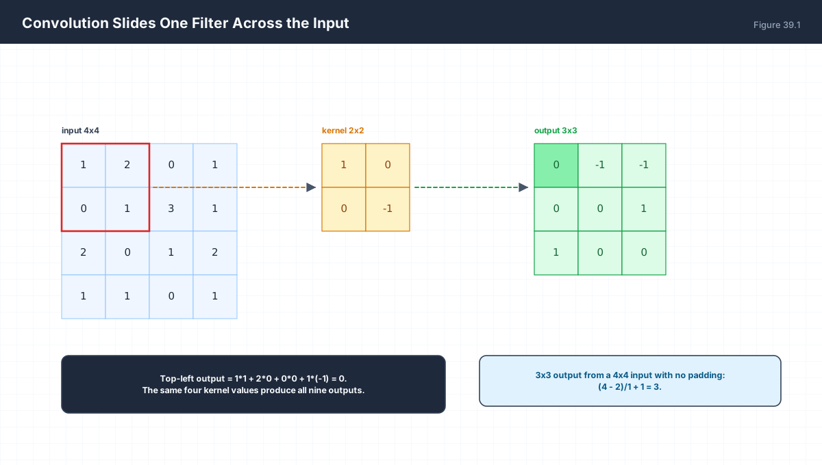
(I * K)[i, j] = sum_{u,v} I[i+u, j+v] K[u, v]

The kernel is placed at every legal offset and dotted
with the patch beneath it. One kernel, many patches.

Strictly this is cross-correlation, not convolution.
Deep learning calls it convolution anyway; the only
difference is a flip of the kernel, which the learned
weights absorb.
import numpy as np

I = np.array([[1, 2, 0, 1],
              [0, 1, 3, 1],
              [2, 0, 1, 2],
              [1, 1, 0, 1]], float)
K = np.array([[1, 0],
              [0, -1]], float)

def conv2d(img, ker):
    kh, kw = ker.shape
    oh, ow = img.shape[0] - kh + 1, img.shape[1] - kw + 1
    out = np.zeros((oh, ow))
    for i in range(oh):
        for j in range(ow):
            out[i, j] = np.sum(img[i:i+kh, j:j+kw] * ker)
    return out

O = conv2d(I, K)
print(O)
print()
print("top-left by hand:", I[0,0]*1 + I[0,1]*0 + I[1,0]*0 + I[1,1]*(-1))
print("matches:", O[0,0] == I[0,0] - I[1,1])

# this kernel is a diagonal edge detector
print("\nabsolute response:", np.abs(O))
The kernel [[1,0],[0,-1]] differences the main diagonal. On a flat region it returns zero; on an edge it returns the jump size. Every CNN filter you ever train is a learned version of exactly this.
3. Deriving the Output Size
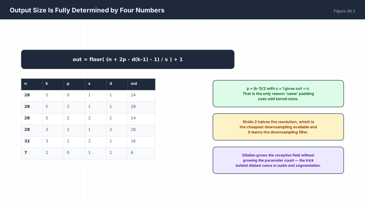
Effective kernel size with dilation d:  d(k-1) + 1
Padded input length:                    n + 2p
Legal placements with stride s:
    floor( (n + 2p - (d(k-1) + 1)) / s ) + 1

p = (k-1)/2 with s = 1 and d = 1 gives out = n,
which is the only reason "same" padding uses odd k.
import math

def out_size(n, k, p=0, s=1, d=1):
    eff = d * (k - 1) + 1
    return (n + 2 * p - eff) // s + 1

cases = [(28, 5, 0, 1, 1), (28, 5, 2, 1, 1), (28, 5, 2, 2, 1),
         (28, 3, 2, 1, 2), (32, 3, 1, 2, 1), (7, 2, 0, 1, 1)]
print(f"{'n':>4}{'k':>4}{'p':>4}{'s':>4}{'d':>4}  {'out':>4}")
for n, k, p, s, d in cases:
    print(f"{n:4d}{k:4d}{p:4d}{s:4d}{d:4d}  {out_size(n,k,p,s,d):4d}")

# 'same' padding really is identity when s = 1
for k in (3, 5, 7, 9):
    p = (k - 1) // 2
    assert out_size(28, k, p) == 28
print("\nsame padding preserves size for odd kernels:", [out_size(28, k, (k-1)//2) for k in (3,5,7,9)])
Every “conv shrinks my tensor” bug is an arithmetic failure in that one line. Stride greater than one is the only case where padding cannot restore the original size.
4. Padding and Border Effects

Without padding, each layer loses k-1 from each side.
Five 3x3 layers on a 32x32 input:
    32 -> 30 -> 28 -> 26 -> 24 -> 22

Interior pixels are touched k^2 times; border pixels
fewer. Zero padding is cheap but introduces an
artificial dark frame the first layer must learn to
ignore. Reflection padding avoids that.
import numpy as np

def shrink(n, layers, k=3, p=0):
    for _ in range(layers):
        n = n - k + 1 + 2 * p
    return n

print("no padding, 5 layers of 3x3 from 32:", shrink(32, 5, 3, 0))
print("same padding, 5 layers of 3x3 from 32:", shrink(32, 5, 3, 1))

# how many output cells does each input position feed?
n, k = 7, 3
oh = n - k + 1
def uses(p, n=n, k=k, oh=oh):
    lo, hi = max(0, p - k + 1), min(p, oh - 1)
    return max(0, hi - lo + 1)

corner = uses(0) * uses(0)
centre = uses(3) * uses(3)
print(f"\ncorner pixel feeds {corner} output cell(s)")
print(f"centre pixel feeds {centre} output cells")
print("ratio:", centre / corner)
A corner pixel feeds exactly one output cell while a centre pixel feeds nine — a 9× imbalance in how much gradient each position receives, and therefore in how well each one is learned. That asymmetry is a real effect, not a cosmetic one, and it is the reason padding choice measurably changes accuracy.
5. Stride and Dilation
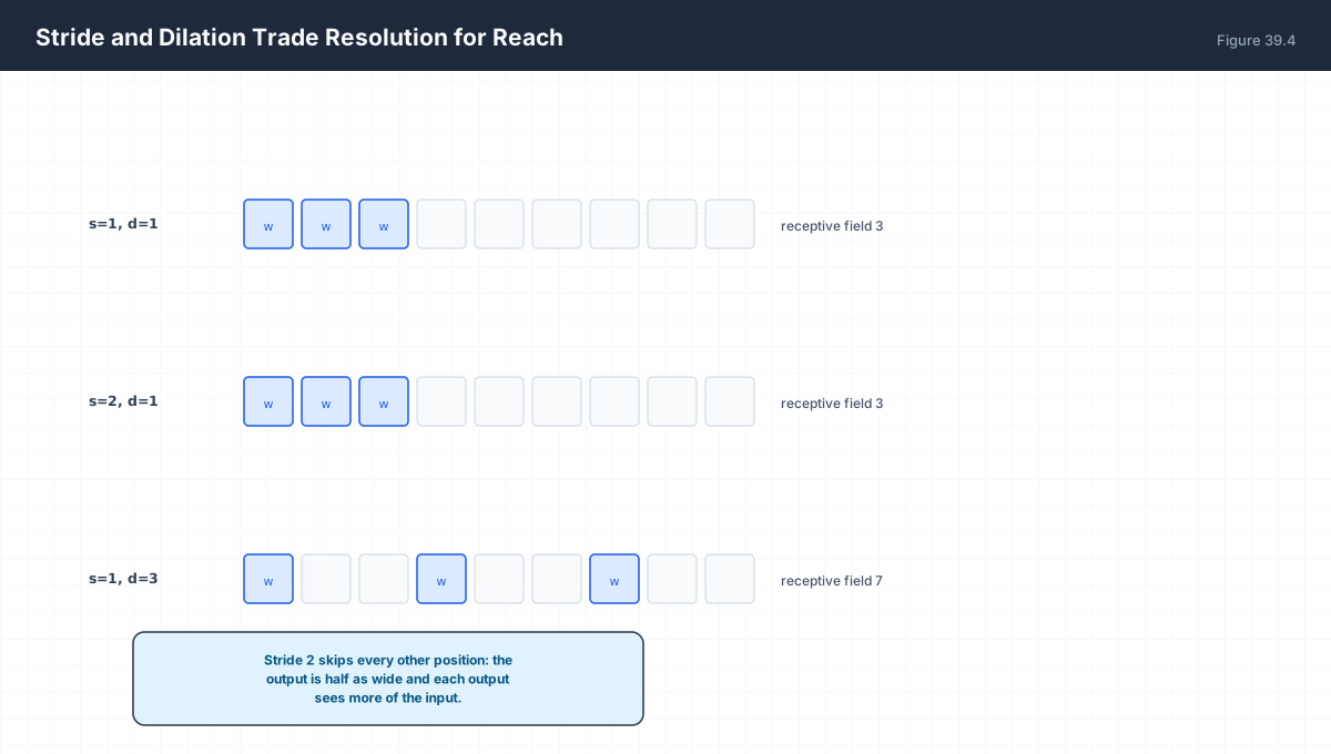
Stride s:  evaluate at every s-th position
           -> output shrinks by ~1/s, receptive field grows

Dilation d: place the k taps d apart
           -> receptive field d(k-1)+1, same k^2 weights

Dilated stacks grow the receptive field exponentially:
d = 1, 2, 4, 8 with k = 3 gives
    3 -> 7 -> 15 -> 31
def receptive_field(dilations, k=3):
    r = 1
    for d in dilations:
        r += (k - 1) * d
    return r

print("plain 3x3 stack:  ", [receptive_field([1]*n) for n in range(1, 6)])
print("dilated 1,2,4,8:  ", receptive_field([1, 2, 4, 8]))
print("same field, plain convs would need", (receptive_field([1,2,4,8]) - 1) // 2, "layers")

for dil in (1, 2, 4):
    eff = dil * (3 - 1) + 1
    print(f"dilation {dil}: effective kernel {eff}x{eff}, weights still {3*3}")
Four dilated layers reach a 31-pixel receptive field using the parameters of four 3×3 convolutions. Two plain layers would reach only 5. This is why dilated convolutions dominate audio, segmentation and time-series work.
6. Weight Sharing and Equivariance

A conv layer with c_in -> c_out channels and k x k taps:
    k^2 * c_in * c_out  weights
  + c_out               biases

A dense layer on the same flattened tensor:
    (H W c_in) * (H W c_out)

Provable property:
    conv(shift(x)) = shift(conv(x))      equivariance

Note this is equivariance, NOT invariance. Shift the
input and the output shifts with it. Invariance only
appears after pooling or global averaging.
import numpy as np

H = W = 64
c_in = c_out = 64
k = 3

conv_p = k * k * c_in * c_out + c_out
dense_p = (H * W * c_in) * (H * W * c_out) + H * W * c_out
print(f"conv  params: {conv_p:>15,}")
print(f"dense params: {dense_p:>15,}")
print(f"ratio: {dense_p/conv_p:,.0f}x")

# equivariance, demonstrated
img = np.zeros((9, 9)); img[4, 4] = 1.0
ker = np.array([[1., 2., 1.], [0., 0., 0.], [-1., -2., -1.]])

def conv2d(a, kk):
    oh, ow = a.shape[0]-kk.shape[0]+1, a.shape[1]-kk.shape[1]+1
    return np.array([[np.sum(a[i:i+kk.shape[0], j:j+kk.shape[1]] * kk)
                      for j in range(ow)] for i in range(oh)])

shifted = np.roll(img, 2, axis=1)
a, b = conv2d(img, ker), conv2d(shifted, ker)
print("\nconv(shift) == shift(conv):", np.allclose(np.roll(a, 2, axis=1), b))
Equivariance holds to machine precision, and it comes for free from the weight sharing — you do not train it in. What you must train is the filter that makes the response meaningful.
7. Worked Examples
7.1 One 3×3 conv on 224×224×3
64 filters of 3x3x3 -> 3*3*3*64 + 64 = 1,792 parameters
output 224*224*64, i.e. 3.2 million activations
7.2 Same layer as a matrix
A conv is a sparse, banded, Toeplitz matrix with tied
entries. Conv layers are dense layers with structure
imposed, not a different operation.
7.3 Receptive field of a plain stack
n layers of k x k with stride 1 given r = n(k-1) + 1.
Ten 3x3 layers reach 21 pixels.
7.4 1×1 convolutions
A 1x1 conv is a dense layer applied per pixel, mixing
channels without looking at neighbours. Width-then-
depth bottlenecks rely on it.
7.5 Depthwise separable convolution
Split k^2*c_in*c_out into k^2*c_in (depthwise) plus
c_in*c_out (pointwise). For k=3 that is roughly a
9x reduction in parameters.
8. Verify It in Python
import numpy as np

def conv2d(a, kk):
    oh, ow = a.shape[0]-kk.shape[0]+1, a.shape[1]-kk.shape[1]+1
    return np.array([[np.sum(a[i:i+kk.shape[0], j:j+kk.shape[1]] * kk)
                      for j in range(ow)] for i in range(oh)])

def out_size(n, k, p=0, s=1, d=1):
    return (n + 2 * p - (d * (k - 1) + 1)) // s + 1

# --- 1. hand-computed values ----------------------------------
I = np.array([[1., 2., 0., 1.], [0., 1., 3., 1.],
              [2., 0., 1., 2.], [1., 1., 0., 1.]])
K = np.array([[1., 0.], [0., -1.]])
O = conv2d(I, K)
assert O.shape == (3, 3)
assert O[0, 0] == 0.0
assert O[0, 1] == 2 - 3
assert np.allclose(O, np.array([[0., -1., -1.], [0., 0., 1.], [1., 0., 0.]]))
print("2-D convolution matches hand arithmetic")

# --- 2. output-size formula -----------------------------------
assert out_size(4, 2) == 3
assert out_size(28, 5, 2) == 28
assert out_size(28, 5, 2, 2) == 14
assert out_size(28, 3, 2, 1, 2) == 28      # dilation 2 needs p = 2
assert out_size(28, 3, 1, 1, 2) == 26      # p = 1 with dilation 2 shrinks
assert out_size(32, 3, 1, 2) == 16
print("output-size formula reproduces all six cases")

# --- 3. formula agrees with actual convolution ----------------
for n, k, p, s in [(9, 3, 0, 1), (9, 3, 1, 1), (9, 3, 1, 2)]:
    a = np.arange(n * n, dtype=float).reshape(n, n)
    ap = np.pad(a, p)
    kk = np.ones((k, k))
    got = conv2d(ap, kk)[::s, ::s]
    assert got.shape == (out_size(n, k, p, s),) * 2, (got.shape, out_size(n, k, p, s))
print("formula matches real convolution output shape")

# --- 4. shift equivariance ------------------------------------
img = np.zeros((10, 10)); img[5, 5] = 1.0
ker = np.array([[1., 2., 1.], [0., 0., 0.], [-1., -2., -1.]])

def shift(a, sh, axis=1):
    """Zero-filled shift. np.roll would WRAP and alias the test."""
    out = np.zeros_like(a)
    if axis == 1:
        out[:, sh:] = a[:, :-sh]
    else:
        out[sh:, :] = a[:-sh, :]
    return out

for sh in (1, 2, 3):
    assert np.allclose(shift(conv2d(img, ker), sh), conv2d(shift(img, sh), ker))
print("conv(shift(x)) == shift(conv(x)) for shifts 1-3 (no wrap)")

# np.roll would have wrapped and produced a false pass/fail
assert not np.allclose(np.roll(conv2d(img, ker), 3, axis=1),
                       conv2d(np.roll(img, 3, axis=1), ker))
print("np.roll wraps, so it is the wrong tool for this test")

# --- 5. borders are visited less often ------------------------
# how many output cells each input position feeds (7x7 input, 3x3 kernel)
def feeds(p, n=7, k=3):
    oh = n - k + 1
    return max(0, min(p, oh - 1) - max(0, p - k + 1) + 1)

assert feeds(0) ** 2 == 1        # corner
assert feeds(3) ** 2 == 9        # centre
assert feeds(1) ** 2 == 4        # near corner
print("corner feeds 1 output, centre feeds 9")

# --- 6. parameter counts --------------------------------------
conv_p = 3 * 3 * 3 * 64 + 64
assert conv_p == 1792
dense_p = (224 * 224 * 3) * (224 * 224 * 64)
print(f"conv params 1,792 vs dense {dense_p:,} — "
      f"{dense_p/conv_p:,.0f}x fewer")

# --- 7. dilation grows the receptive field --------------------
def rf(dils, k=3):
    r = 1
    for d in dils:
        r += (k - 1) * d
    return r

assert rf([1]) == 3 and rf([1, 1]) == 5
assert rf([1, 2, 4, 8]) == 31
assert rf([1, 2, 4, 8]) == rf([1] * 15)
print("four dilated layers == fifteen plain layers in reach")

# --- 8. 1x1 conv is a per-pixel dense layer -------------------
X = np.random.default_rng(0).normal(size=(6, 6, 3))
W1 = np.random.default_rng(1).normal(size=(4, 3))
via_dense = X @ W1.T
manual = np.array([[[np.sum(X[i, j] * W1[o]) for o in range(4)]
                    for j in range(6)] for i in range(6)])
assert np.allclose(via_dense, manual)
print("1x1 conv across channels == dense layer per pixel")
print("all assertions passed")
9. Practice Questions
- Compute a 2-D convolution of a 5×5 input with a 3×3 kernel by hand.
- Derive the output-size formula.
- Why does “same” padding require an odd kernel size?
- What does stride 2 do to the output resolution?
- How much does dilation 3 grow a 3×3 kernel’s receptive field?
- Distinguish equivariance from invariance.
- Count the parameters of a 3×3×32→64 convolution.
- Why is a 1×1 convolution useful?
- Compute the receptive field of six 3×3 layers.
- Explain why a stacked conv net is not a dense net with fewer parameters.
10. Official References & Further Reading
Continue the Course
- Course Index: AI Mathematics Masterclass — All 48 Chapters
- Previous Chapter: Chapter 38: Activation Functions & Nonlinearity
- Next Chapter: Chapter 40: Sequence Models & Positional Encoding Mathematics
- Related Series: PyTorch Engineering Masterclass — All 16 Modules