
AI Reading
Quick summary of this article
AI Mathematics Masterclass — Chapter 33 of 48
Correlation and regression are the two oldest tools in applied statistics, and the two most frequently misread. Correlation measures only linear association and says nothing about causation; regression fits a conditional mean and says nothing about the individual case. This chapter derives both from covariance, shows why the least-squares line has the form it does, and explains how residual plots reveal what the fit missed.
1. Technical Audit & Core Learning Objectives
| Component | Common Tutorial Deficiency | Engineering Standard Applied Here |
|---|---|---|
| Correlation | Presented as “how related two things are”. | Restricted explicitly to linear association, with a zero-correlation curve counterexample. |
| Regression | Formula given without deriving slope from covariance. | Slope derived as Cov/Var, matching the projection argument of Chapter 12. |
| Diagnostics | R² reported alone. | Residual plots shown for the three standard failure patterns. |
| Aggregation | Simpson’s paradox never mentioned. | Shown as a case where pooling reverses a within-group trend. |
Core learning objectives. After this chapter you should be able to:
- Compute Pearson correlation and state its range and limits.
- Give an example of zero correlation with a strong relationship.
- Derive the least-squares slope as
Cov(x,y)/Var(x). - Show that the fitted line passes through the point of means.
- Read a residual plot and name the misspecification it reveals.
- Explain Simpson’s paradox and why stratification changes conclusions.
2. Correlation Is Linear Only
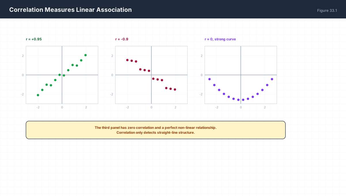
Pearson r = Cov(x, y) / (SD(x) SD(y))        range [-1, 1]

r = 0 means no LINEAR association.
It does not mean independence — see y = x^2.

Spearman rank correlation catches monotone non-linear
relationships that Pearson misses.
import numpy as np

rng = np.random.default_rng(0)
x = rng.uniform(-3, 3, 20000)
y_lin = 2 * x + rng.normal(0, 0.5, x.size)
y_quad = x ** 2 + rng.normal(0, 0.3, x.size)

print("linear  : r =", round(np.corrcoef(x, y_lin)[0, 1], 4))
print("quadratic: r =", round(np.corrcoef(x, y_quad)[0, 1], 4), "  <- near zero")

# a rank correlation would be needed to detect the monotone half;
# Pearson cannot, by construction
The quadratic case is the standard demonstration that r = 0 does not mean "unrelated". It means "no straight line summarises this". Reporting correlation without plotting is how that error survives.
3. Least Squares From Covariance
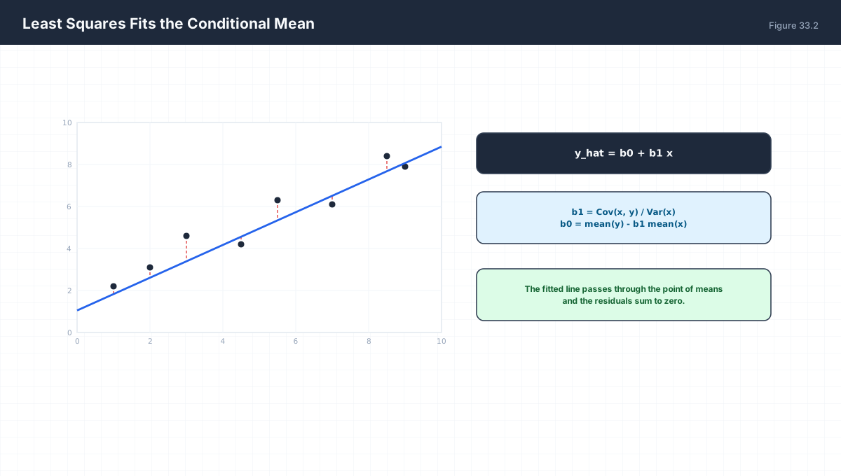
minimise  sum (y_i - b0 - b1 x_i)^2

b1 = Cov(x, y) / Var(x)
b0 = mean(y) - b1 mean(x)

Consequences:
  the line passes through (mean x, mean y)
  the residuals sum to zero
  r^2 = b1^2 Var(x) / Var(y)
import numpy as np

rng = np.random.default_rng(1)
x = rng.normal(0, 1, 500)
y = 3.0 * x + 2.0 + rng.normal(0, 0.5, 500)

b1 = np.cov(x, y, ddof=0)[0, 1] / x.var()
b0 = y.mean() - b1 * x.mean()
print(f"fitted: y = {b1:.3f} x + {b0:.3f}   (true 3.0, 2.0)")

resid = y - (b0 + b1 * x)
print("sum of residuals:", round(resid.sum(), 10))
print("mean point on line:", np.isclose(b0 + b1 * x.mean(), y.mean()))

# cross-check against lstsq
X = np.column_stack([x, np.ones_like(x)])
w, *_ = np.linalg.lstsq(X, y, rcond=None)
assert np.allclose(w, [b1, b0], atol=1e-9)
print("matches lstsq")
This is the same solution derived in Chapter 12 by projection. The normal equations XᵀX w = Xᵀy reduce to the covariance formulas in the single-predictor case — a useful consistency check that the geometry and the algebra agree.
4. Residual Plots
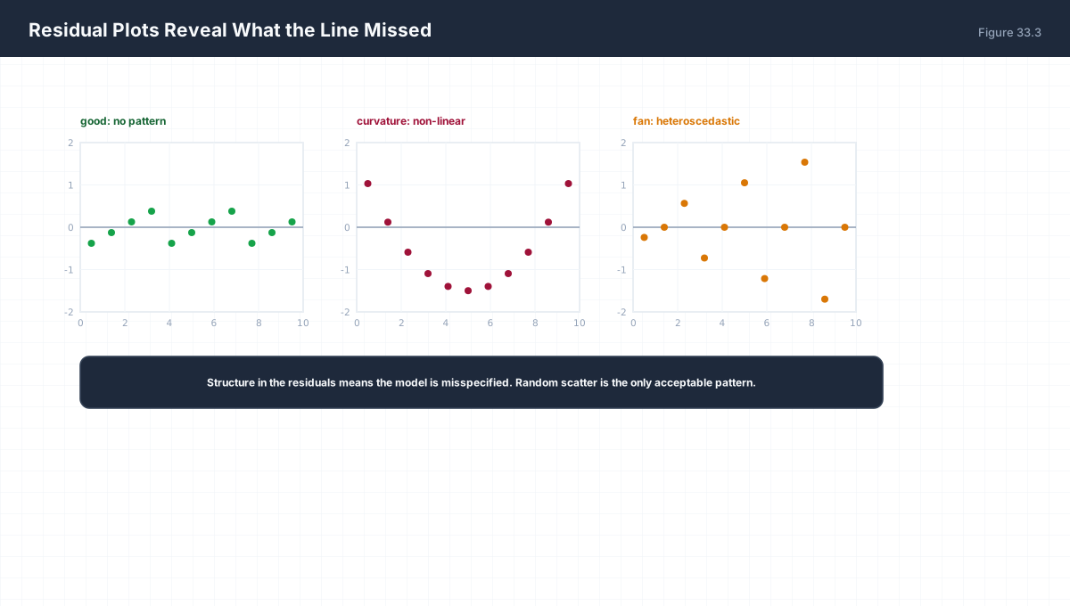
| Pattern | Diagnosis | Fix |
|---|---|---|
| Random scatter | Model is adequate | None |
| Curvature (U or arch) | Relationship is non-linear | Add a polynomial or transform |
| Fan shape | Heteroscedasticity — variance depends on x | Weighted least squares or log-transform |
import numpy as np

rng = np.random.default_rng(2)
x = np.linspace(0, 10, 400)

# heteroscedastic: noise grows with x
y = 2 * x + rng.normal(0, 1, x.size) * (0.2 + x * 0.3)
X = np.column_stack([x, np.ones_like(x)])
w, *_ = np.linalg.lstsq(X, y, rcond=None)
resid = y - X @ w

# bucket the residuals and compare their spread
buckets = np.array_split(resid, 5)
print("residual std by bucket:", [round(b.std(), 3) for b in buckets])
print("spread grows left to right -> heteroscedasticity")
5. R² and Its Limits

import numpy as np

rng = np.random.default_rng(3)
n = 100
x = rng.normal(size=(n, 1))
y = rng.normal(size=n)               # pure noise, no relationship

def r2(X, y):
    X1 = np.column_stack([X, np.ones(len(y))])
    w, *_ = np.linalg.lstsq(X1, y, rcond=None)
    pred = X1 @ w
    ss_res = ((y - pred) ** 2).sum()
    ss_tot = ((y - y.mean()) ** 2).sum()
    return 1 - ss_res / ss_tot

print(f"R^2 with 1 noise feature : {r2(x, y):.4f}")
X_many = rng.normal(size=(n, 30))
print(f"R^2 with 30 noise features: {r2(X_many, y):.4f}")
print("R^2 rises with irrelevant features — it always does")
With 30 random predictors and 100 samples, R² climbs to roughly 0.3 despite there being no relationship whatsoever. Adjusted R² and cross-validation penalise this; a raw in-sample R² on a model with many parameters is close to meaningless.
6. Simpson's Paradox
import numpy as np

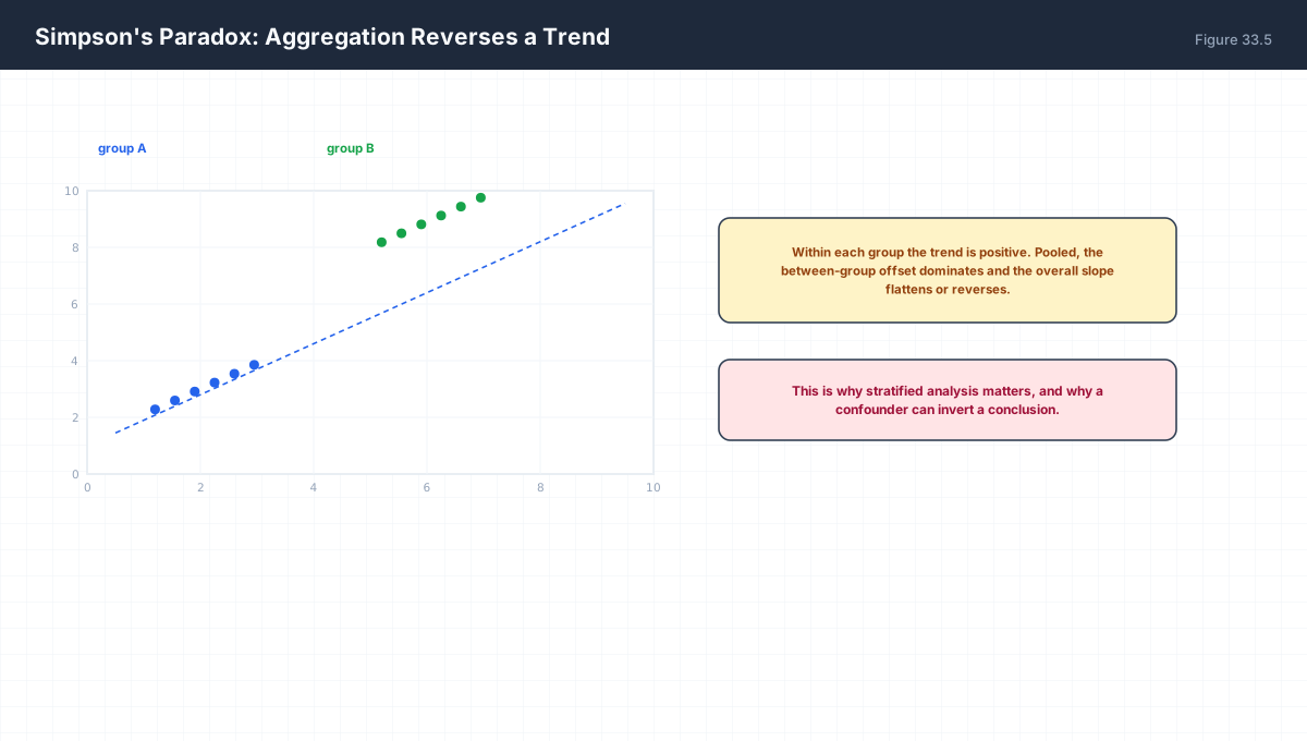
# each group rises internally, but the groups sit at opposite heights
g1x = np.array([1., 2., 3., 4.]); g1y = np.array([10.0, 10.9, 12.1, 12.8])
g2x = np.array([6., 7., 8., 9.]); g2y = np.array([2.0, 2.9, 4.1, 4.8])

def slope(x, y):
    return np.cov(x, y, ddof=0)[0, 1] / x.var()

print("group 1 slope:", round(slope(g1x, g1y), 3))
print("group 2 slope:", round(slope(g2x, g2y), 3))
print("pooled slope :", round(slope(np.r_[g1x, g2x], np.r_[g1y, g2y]), 3))
Both groups rise. Pooled, the trend reverses, because the between-group offset dominates the within-group relationship. Any analysis that ignores a group label correlated with both variables can report the opposite sign to the truth — which is why stratifying before concluding is not optional.
7. Worked Examples
7.1 Correlation from covariance
Cov(x,y) = 6,  SD(x) = 3,  SD(y) = 4
r = 6 / 12 = 0.5
7.2 Slope from correlation
b1 = r * SD(y) / SD(x) = 0.5 * 4 / 3 = 0.667
7.3 R² from correlation
For simple linear regression, R^2 = r^2.
r = 0.5 -> R^2 = 0.25, so 25% of variance explained.
7.4 Intercept
mean(x) = 5, mean(y) = 10, b1 = 0.667
b0 = 10 - 0.667*5 = 6.67
7.5 Why not regress x on y
Regressing x on y gives a different slope: r SD(x)/SD(y).
Ordinary least squares minimises vertical error only,
so the direction of regression is a choice, not a formality.
8. Verify It in Python
import numpy as np

rng = np.random.default_rng(0)

# --- 1. correlation bounds ---------------------------------------
for _ in range(50):
    a = rng.normal(size=200); b = rng.normal(size=200)
    r = np.corrcoef(a, b)[0, 1]
    assert -1.0001 <= r <= 1.0001
print("correlation stays in [-1, 1]")

# --- 2. zero correlation with dependence -------------------------
x = rng.uniform(-3, 3, 30000)
assert abs(np.corrcoef(x, x ** 2)[0, 1]) < 0.05
print("corr(x, x^2) ~ 0 despite exact dependence")

# --- 3. slope equals Cov/Var ------------------------------------
xv = rng.normal(0, 2, 800)
yv = -1.5 * xv + 4 + rng.normal(0, 0.4, 800)
b1 = np.cov(xv, yv, ddof=0)[0, 1] / xv.var()
assert abs(b1 + 1.5) < 0.05
print("slope recovered:", round(b1, 3))

# --- 4. line passes through the means ---------------------------
b0 = yv.mean() - b1 * xv.mean()
assert np.isclose(b0 + b1 * xv.mean(), yv.mean())
print("line passes through the mean point")

# --- 5. residuals sum to zero -----------------------------------
resid = yv - (b0 + b1 * xv)
assert abs(resid.sum()) < 1e-9
print("residuals sum to zero")

# --- 6. R^2 == r^2 for simple regression ------------------------
r = np.corrcoef(xv, yv)[0, 1]
ss_res = (resid ** 2).sum()
ss_tot = ((yv - yv.mean()) ** 2).sum()
assert np.isclose(1 - ss_res / ss_tot, r ** 2, atol=1e-9)
print("R^2 equals r^2:", round(r**2, 4))

# --- 7. R^2 inflates with noise features ------------------------
n = 120
noise_y = rng.normal(size=n)

def r2(X, y):
    X1 = np.column_stack([X, np.ones(len(y))])
    w, *_ = np.linalg.lstsq(X1, y, rcond=None)
    pred = X1 @ w
    return 1 - ((y - pred) ** 2).sum() / ((y - y.mean()) ** 2).sum()

r2_one = r2(rng.normal(size=(n, 1)), noise_y)
r2_many = r2(rng.normal(size=(n, 30)), noise_y)
assert r2_many > r2_one + 0.1
print(f"R^2 with 1 vs 30 noise features: {r2_one:.3f} -> {r2_many:.3f}")

# --- 8. Simpson's paradox is reproducible -----------------------
g1x = np.array([1., 2., 3., 4.]); g1y = np.array([10., 10.9, 12.1, 12.8])
g2x = np.array([6., 7., 8., 9.]); g2y = np.array([2., 2.9, 4.1, 4.8])
slope = lambda a, b: np.cov(a, b, ddof=0)[0, 1] / a.var()
assert slope(g1x, g1y) > 0 and slope(g2x, g2y) > 0   # both rise within group
assert slope(np.r_[g1x, g2x], np.r_[g1y, g2y]) < 0   # pooled trend reverses
print("within-group slopes:", round(slope(g1x,g1y),2), round(slope(g2x,g2y),2),
      " pooled:", round(slope(np.r_[g1x,g2x], np.r_[g1y,g2y]),2))
print("all assertions passed")
9. Practice Questions
- Compute the Pearson correlation given
Cov=6,SD(x)=3,SD(y)=4. - Give an example of zero correlation with a strong relationship.
- Derive the least-squares slope in terms of covariance and variance.
- Show that the fitted line passes through the mean point.
- Why do the residuals of a fitted line sum to zero?
- State the relation between R² and r for simple regression.
- Interpret a fan-shaped residual plot.
- Why does R² rise when noise features are added?
- Explain Simpson's paradox and its practical warning.
- Why is regressing x on y different from y on x?
10. Official References & Further Reading
Continue the Course
- Course Index: AI Mathematics Masterclass — All 48 Chapters
- Previous Chapter: Chapter 32: Hypothesis Testing & Confidence Intervals
- Next Chapter: Chapter 34: Bias–Variance Tradeoff & Regularization Mathematics
- Related Series: PyTorch Engineering Masterclass — All 16 Modules