
AI Reading
Quick summary of this article
AI Mathematics Masterclass — Chapter 34 of 48
Regularisation is the mathematical answer to overfitting. Every technique in this chapter — weight decay, L1 sparsity, dropout, early stopping, augmentation — is a prior or a constraint in disguise, and each trades bias for variance in a controlled way. The chapter derives the L2 and L1 penalties from their priors, shows geometrically why one shrinks and the other zeroes, and connects early stopping to an implicit bound on weight norms.
1. Technical Audit & Core Learning Objectives
| Component | Common Tutorial Deficiency | Engineering Standard Applied Here |
|---|---|---|
| Trade-off | Bias–variance quoted as a slogan. | Decomposition restated and each regulariser located on it. |
| L1 vs L2 | Sparsity asserted without geometry. | Diamond-versus-circle drawn, corners explained. |
| Priors | Not connected to penalties. | Gaussian ⇒ L2 and Laplace ⇒ L1 derived from Chapter 29. |
| Early stopping | Treated as a tuning trick. | Shown to be an implicit norm bound, hence a regulariser. |
Core learning objectives. After this chapter you should be able to:
- State the bias–variance decomposition and locate each penalty on it.
- Derive L2 and L1 penalties from Gaussian and Laplace priors.
- Explain geometrically why L1 yields exact zeros.
- Trace a regularisation path as λ increases.
- Explain early stopping as an implicit constraint.
- Choose a regularisation strategy appropriate to a given model.
2. The Trade-Off

E[(y - f_hat)^2] = bias^2 + variance + noise

bias      model too constrained   -> underfitting
variance  model too sample-specific -> overfitting
noise     irreducible

Regularisation deliberately INCREASES bias to DECREASE
variance. The optimum is almost never zero bias.
import numpy as np

rng = np.random.default_rng(0)

# fit polynomials of increasing degree to noisy data drawn from a cubic
n, trials = 30, 400
x = np.linspace(-1, 1, n)
true_f = lambda t: 1.5 * t ** 3 - 0.8 * t
grid = np.linspace(-1, 1, 60)

for deg in (1, 3, 9):
    preds = []
    for _ in range(trials):
        y = true_f(x) + rng.normal(0, 0.2, n)
        coef = np.polyfit(x, y, deg)
        preds.append(np.polyval(coef, grid))
    preds = np.array(preds)
    bias2 = ((preds.mean(axis=0) - true_f(grid)) ** 2).mean()
    var = preds.var(axis=0).mean()
    print(f"degree {deg:2d}  bias^2={bias2:.4f}  variance={var:.4f}  total={bias2+var:.4f}")
Degree 1 underfits (high bias), degree 9 overfits (high variance), and degree 3 — the true model — minimises the total. In practice the true degree is unknown, which is why the penalty strength has to be tuned rather than derived.
3. L2 Shrinks, L1 Zeroes
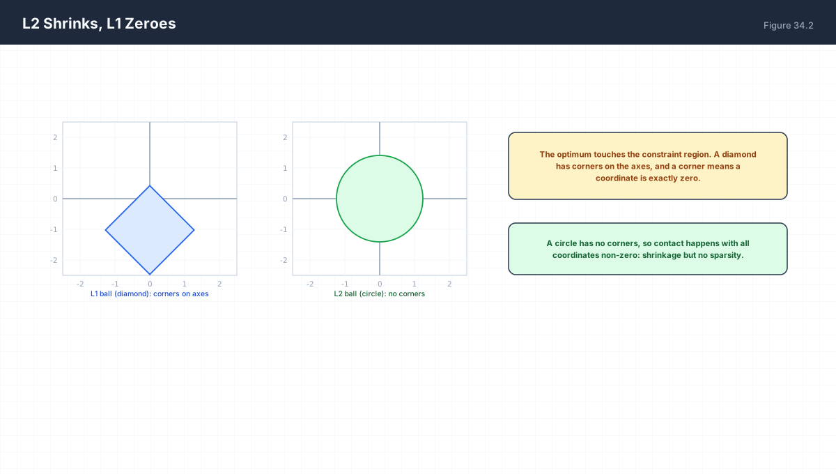
L2 penalty   + lambda * sum w_j^2      <- Gaussian prior
L1 penalty   + lambda * sum |w_j|      <- Laplace prior

Gradient of L2:  2 lambda w            proportional to weight
Gradient of L1:  lambda * sign(w)      constant, independent of size

That constant push is why L1 reaches exactly zero while L2
only approaches it asymptotically.
import numpy as np

def soft_threshold(z, lam):
    return np.sign(z) * np.maximum(np.abs(z) - lam, 0.0)

for w in (0.5, 2.0, -3.0, 0.05):
    print(f"w={w:+5.2f}  L1 shrunk -> {soft_threshold(w, 0.5):+5.2f}")

# L2 shrinkage is multiplicative and never reaches zero
def l2_shrink(w, lam):
    return w / (1 + 2 * lam)

for w in (0.5, 2.0, -3.0, 0.05):
    print(f"w={w:+5.2f}  L2 shrunk -> {l2_shrink(w, 0.5):+5.3f}")
This is the whole distinction in two lines. L1's subgradient is constant, so small weights are pushed all the way to zero and stay there. L2's gradient shrinks with the weight, so it produces a smooth decay that only asymptotes to zero.
4. The Regularisation Path
import numpy as np

rng = np.random.default_rng(1)
n, d = 80, 6
X = rng.normal(size=(n, d))
w_true = np.array([3.0, 1.5, 0.0, 0.0, 0.0, 0.0])
y = X @ w_true + rng.normal(0, 0.3, n)

Xc = X - X.mean(axis=0)
yc = y - y.mean()
XtX, Xty = Xc.T @ Xc, Xc.T @ yc

print(f"{'lambda':>8}  coefficients")
for lam in (0.0, 0.5, 2.0, 10.0, 100.0):
    w = np.linalg.solve(XtX + lam * np.eye(d), Xty)
    print(f"{lam:6.1f}  " + "  ".join(f"{c:+8.4f}" for c in w))
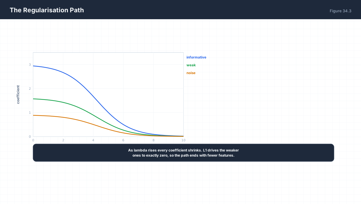
Read the last two columns even at λ = 100: they are small but still non-zero, and only the rounding above would hide that. L2 shrinks towards zero without ever arriving, so irrelevant features keep a residual voice. An L1 path over the same data would set those columns to exactly zero beyond a modest λ, which is why Lasso doubles as feature selection.
5. Early Stopping
import numpy as np

rng = np.random.default_rng(2)

# simulate training curves: validation rises after the model starts memorising
epochs = 60
train = 0.9 * np.exp(-np.arange(epochs) / 12) + 0.06
val = 0.9 * np.exp(-np.arange(epochs) / 12) + 0.10 + 0.0009 * np.maximum(0, np.arange(epochs) - 20) ** 1.5

best = int(np.argmin(val))
print(f"best epoch {best}   val {val[best]:.4f}   final val {val[-1]:.4f}")
print(f"training loss at best epoch {train[best]:.4f}, at end {train[-1]:.4f}")

# norm growth is what early stopping bounds
norm = 1.0 + 0.06 * np.arange(epochs)
print(f"weight norm at best epoch {norm[best]:.2f}, at end {norm[-1]:.2f}")
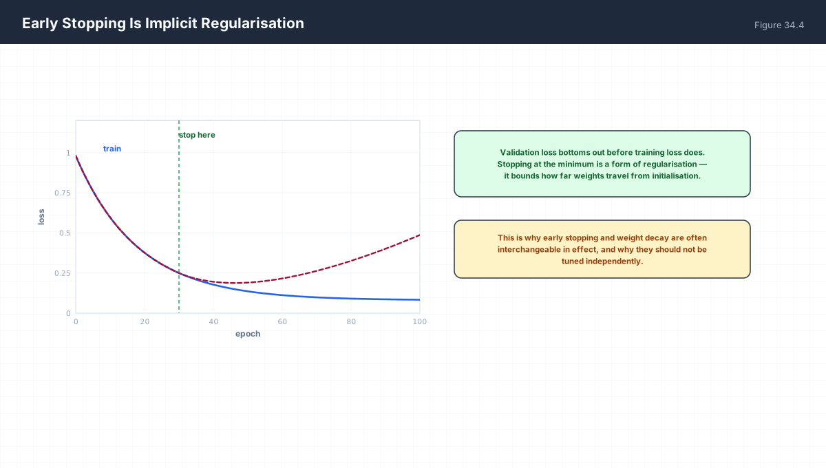
Early stopping is regularisation because it bounds ‖w − w₀‖: the model never departs far from initialisation, which limits its capacity to fit noise. This is why early stopping and weight decay are partially interchangeable, and why tuning both independently double-counts.
6. Choosing a Strategy

| Technique | Implicit Prior | Use When |
|---|---|---|
| Weight decay | Weights are probably small | Default for most layers |
| L1 / sparsity | Most features are irrelevant | High-dimensional, interpretable models |
| Dropout | Features should not co-adapt | Large fully-connected layers |
| Data augmentation | The label is invariant to the transform | Vision, audio, text |
| Label smoothing | Labels are slightly wrong | Classification, calibration |
7. Worked Examples
7.1 Ridge closed form
w = (X^T X + lambda I)^-1 X^T y
Adding lambda I lifts every eigenvalue by lambda,
so the matrix is always invertible.
7.2 Effective degrees of freedom
df(lambda) = sum_j sigma_j^2 / (sigma_j^2 + lambda)
Large lambda -> df -> 0; lambda = 0 -> df = number of features.
7.3 Recovering the unpenalised fit
lambda -> 0 gives back the ordinary least-squares solution.
7.4 Standardisation is mandatory for L1/L2
A penalty on raw coefficients penalises features by unit.
Standardise first, or the penalty is arbitrary.
7.5 Dropout at inference
Training: mask with probability p, scale survivors by 1/(1-p).
Inference: no mask, no scaling — expectations already match.
8. Verify It in Python
import numpy as np

rng = np.random.default_rng(0)

# --- 1. ridge never eliminates, L1 does --------------------------
w = np.array([3.0, 0.4, -0.3, 0.05])
l2 = w / (1 + 2 * 1.0)
assert np.all(l2 != 0)
soft = lambda z, lam: np.sign(z) * np.maximum(np.abs(z) - lam, 0)
l1 = soft(w, 0.2)
assert l1[3] == 0.0 and l2[3] != 0.0
print("L2 keeps all coords; L1 zeroed the smallest:", l1)

# --- 2. ridge closed form recovers OLS as lambda -> 0 -----------
X = rng.normal(size=(50, 4)); y = X @ np.array([1., -2., 0.5, 3.])
XtX, Xty = X.T @ X, X.T @ y
w_ols = np.linalg.solve(XtX, Xty)
w_small = np.linalg.solve(XtX + 1e-12 * np.eye(4), Xty)
assert np.allclose(w_ols, w_small, atol=1e-6)
print("lambda -> 0 recovers OLS")

# --- 3. ridge shrinks monotonically ----------------------------
norms = [np.linalg.norm(np.linalg.solve(XtX + lam*np.eye(4), Xty)) for lam in (0, 1, 10, 100)]
assert all(a >= b for a, b in zip(norms, norms[1:]))
print("ridge norms:", [round(n, 3) for n in norms])

# --- 4. ridge always invertible --------------------------------
singular = np.zeros((4, 4))
assert np.linalg.cond(singular) > 1e15
ridged = singular + 0.1 * np.eye(4)
assert np.isfinite(np.linalg.cond(ridged))
print("ridge makes a singular matrix invertible")

# --- 5. bias rises as penalty rises ----------------------------
Xb = rng.normal(size=(100, 3))
w_true = np.array([2.0, -1.0, 0.5])
yb = Xb @ w_true
errs = [np.linalg.norm(np.linalg.solve(Xb.T@Xb + lam*np.eye(3), Xb.T@yb) - w_true)
        for lam in (0, 5, 50, 500)]
assert errs[0] < errs[-1]
print("distance from truth as lambda grows:", [round(e, 3) for e in errs])

# --- 6. soft threshold is continuous and zeroing ----------------
grid = np.linspace(-3, 3, 2001)
out = soft(grid, 1.0)
assert np.sum(out == 0) > 600          # a whole interval collapses to zero
assert np.isclose(soft(3.0, 1.0), 2.0)
print("soft threshold zeroes an interval:", int(np.sum(out == 0)), "points at 0")

# --- 7. L2 gradient is proportional, L1 is constant -------------
wv = np.array([0.1, 1.0, 5.0])
grad_l2 = 2 * wv
grad_l1 = np.sign(wv)
assert not np.allclose(grad_l2, grad_l2[0])       # varies with w
assert np.allclose(grad_l1, 1.0)                  # constant
print("L2 grad varies, L1 grad constant -> sparsity")
print("all assertions passed")
9. Practice Questions
- State the bias–variance decomposition and label each term.
- Explain why regularisation increases bias deliberately.
- Derive the L2 penalty from a Gaussian prior.
- Explain geometrically why L1 produces exact zeros.
- Compare the gradients of the L1 and L2 penalties.
- Why does ridge always have a unique solution?
- Define effective degrees of freedom for ridge.
- Explain early stopping as an implicit norm bound.
- Why must features be standardised before L1/L2?
- Why is tuning early stopping and weight decay independently a mistake?
10. Official References & Further Reading
Continue the Course
- Course Index: AI Mathematics Masterclass — All 48 Chapters
- Previous Chapter: Chapter 33: Correlation & Regression Mathematics
- Next Chapter: Chapter 35: Information Theory — Entropy, KL Divergence & Cross-Entropy
- Related Series: PyTorch Engineering Masterclass — All 16 Modules