
AI Reading
Quick summary of this article
AI Mathematics Masterclass — Chapter 9 of 48
A matrix carries two readings at once. As data it is a table: rows are samples, columns are features. As an operator it is a function that maps one vector space to another. Almost every confusion in applied linear algebra comes from mixing those two readings. This chapter builds both, catalogues the special matrices worth recognising on sight, and explains rank as the precise statement of how much information an operator destroys.
1. Technical Audit & Core Learning Objectives
Matrices are usually introduced as grids of numbers with elementwise operations, and the operator reading arrives too late — often never. That ordering produces practitioners who can add matrices but cannot explain why a weight matrix’s shape is (d_out × d_in).
| Component | Common Tutorial Deficiency | Engineering Standard Applied Here |
|---|---|---|
| Two readings | Only the table reading is taught. | Data and operator readings developed side by side and explicitly contrasted. |
| Special matrices | Identity and diagonal mentioned; symmetric, orthogonal, triangular omitted. | The full set that appears in real architectures. |
| Transpose | Defined mechanically, with the product-reversal rule glossed over. | (AB)ᵀ = BᵀAᵀ derived and used in backpropagation. |
| Rank | Defined as a row count, with no link to information loss. | Rank framed as the dimension of the image — exactly what an operator preserves. |
Core learning objectives. After this chapter you should be able to:
- State the shape, size, row, column, and element of a matrix and index each correctly.
- Recognise identity, diagonal, symmetric, orthogonal, triangular, and zero matrices.
- Add, scale, and transpose matrices, and apply
(AB)ᵀ = BᵀAᵀ. - Compute rank and state what a rank deficiency means for a layer.
- Distinguish a data matrix from an operator matrix and justify the shape of a weight matrix.
- Explain why an orthogonal matrix has a free inverse.
2. Anatomy
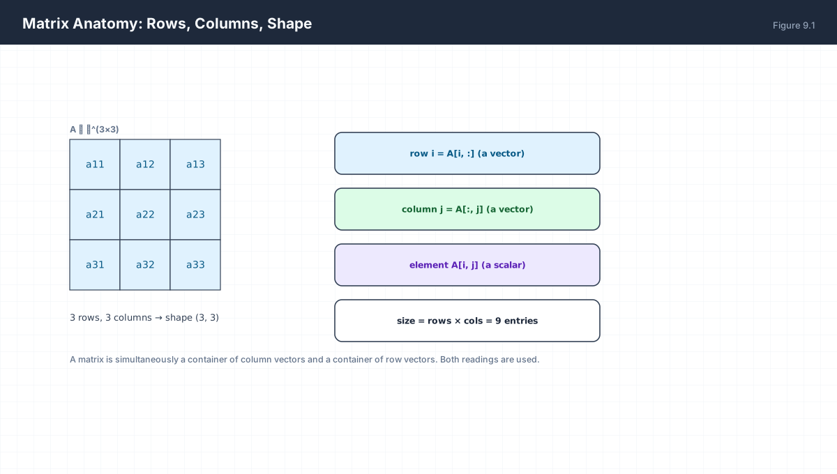
A ∈ ℝ^(m×n)        m rows, n columns, m·n entries
A[i, :]            row i    — a vector of length n
A[:, j]            column j — a vector of length m
A[i, j]            one element — a scalar
import numpy as np

A = np.arange(1, 10, dtype=float).reshape(3, 3)
print(A.shape, A.size)         # (3, 3) 9
print("row 1   :", A[1, :])
print("column 2:", A[:, 2])
print("element :", A[1, 2])
NumPy is 0-indexed while mathematical writing is usually 1-indexed. Off-by-one errors in matrix indexing are common and almost always silent — they return a valid number from the wrong place rather than raising.
3. Special Matrices
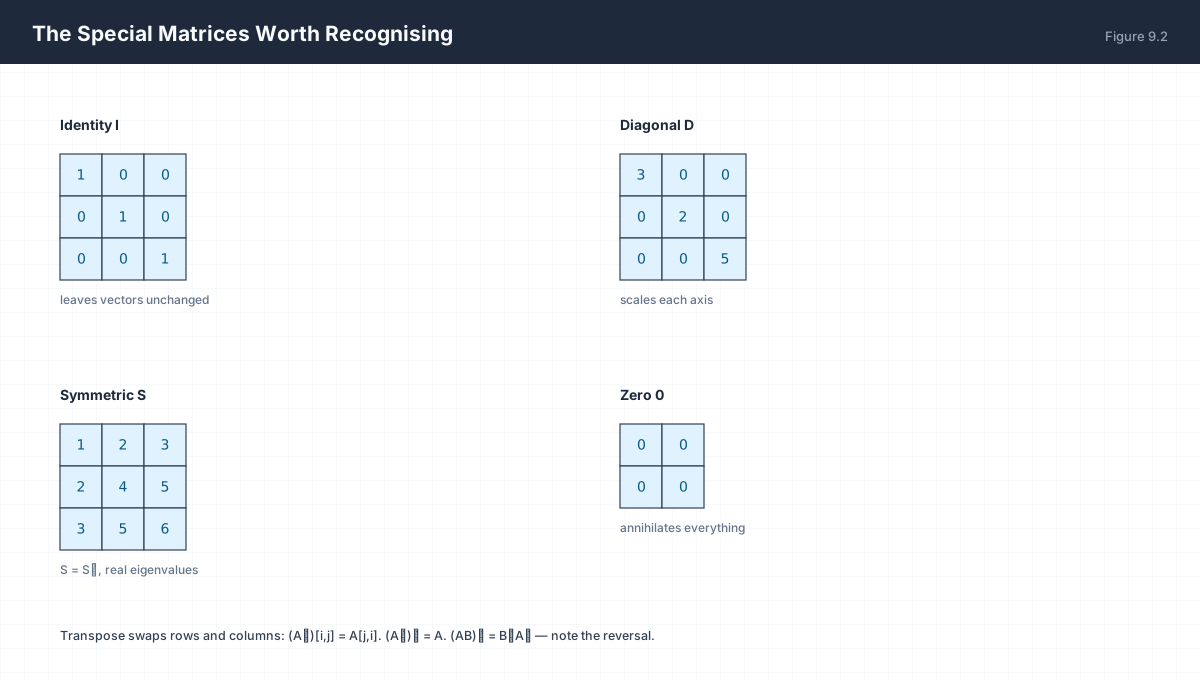
| Matrix | Property | Where It Appears |
|---|---|---|
Identity I |
AI = IA = A |
Residual connections, initialisation |
Diagonal D |
Scales each axis independently | Per-channel scaling, attention masks |
Symmetric S = Sᵀ |
Real eigenvalues, orthogonal eigenvectors | Covariance matrices, Hessians |
Orthogonal QᵀQ = I |
Q⁻¹ = Qᵀ, preserves lengths |
Rotation, Householder reflections, QR |
Triangular L, U |
Solvable by substitution | LU factorisation, causal attention masks |
The orthogonal case deserves attention because it is the cheapest structural win available. Since QᵀQ = I, the inverse is a transpose — an operation that costs nothing. Weights are sometimes re-parameterised to stay orthogonal precisely so that gradients neither explode nor vanish across many layers.
4. Elementwise Operations and the Transpose
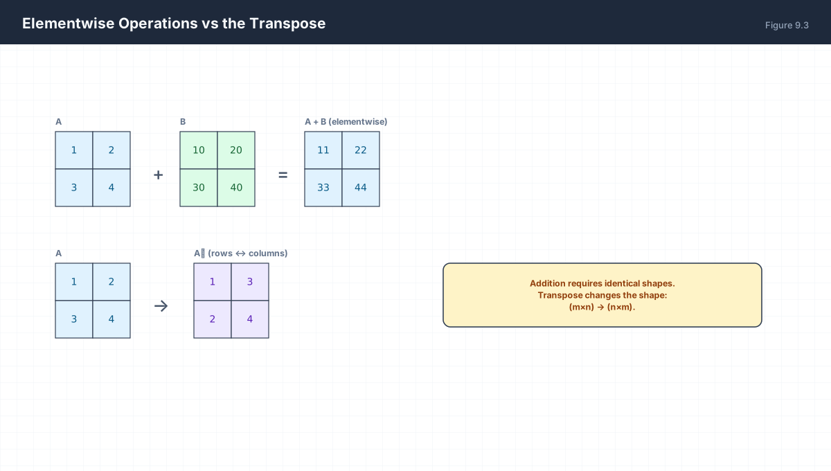
Elementwise:  (A + B)[i,j] = A[i,j] + B[i,j]      requires identical shape
Scaling:      (cA)[i,j]    = c · A[i,j]
Hadamard:     (A ⊙ B)[i,j] = A[i,j] · B[i,j]     elementwise product, same shape

Transpose:    (Aᵀ)[i,j] = A[j,i]                 (m×n) → (n×m)
              (Aᵀ)ᵀ = A
              (A + B)ᵀ = Aᵀ + Bᵀ
              (AB)ᵀ = BᵀAᵀ          ← order reverses
import numpy as np

A = np.array([[1., 2.], [3., 4.]])
B = np.array([[10., 20.], [30., 40.]])

print("A + B      :\n", A + B)
print("A * B (had):\n", A * B)          # elementwise, NOT matrix product
print("A @ B      :\n", A @ B)          # true matrix product

M = np.random.rand(2, 3)
assert (M.T).shape == (3, 2)
assert np.allclose((M.T).T, M)

X = np.random.rand(2, 3); Y = np.random.rand(3, 4)
assert np.allclose((X @ Y).T, Y.T @ X.T)     # the reversal rule
print("transpose reversal verified")
The distinction between * and @ is the single most common NumPy bug. * is the Hadamard product; @ is the matrix product. In attention masks you want *; in a layer you want @.
5. Rank: How Much Information Survives
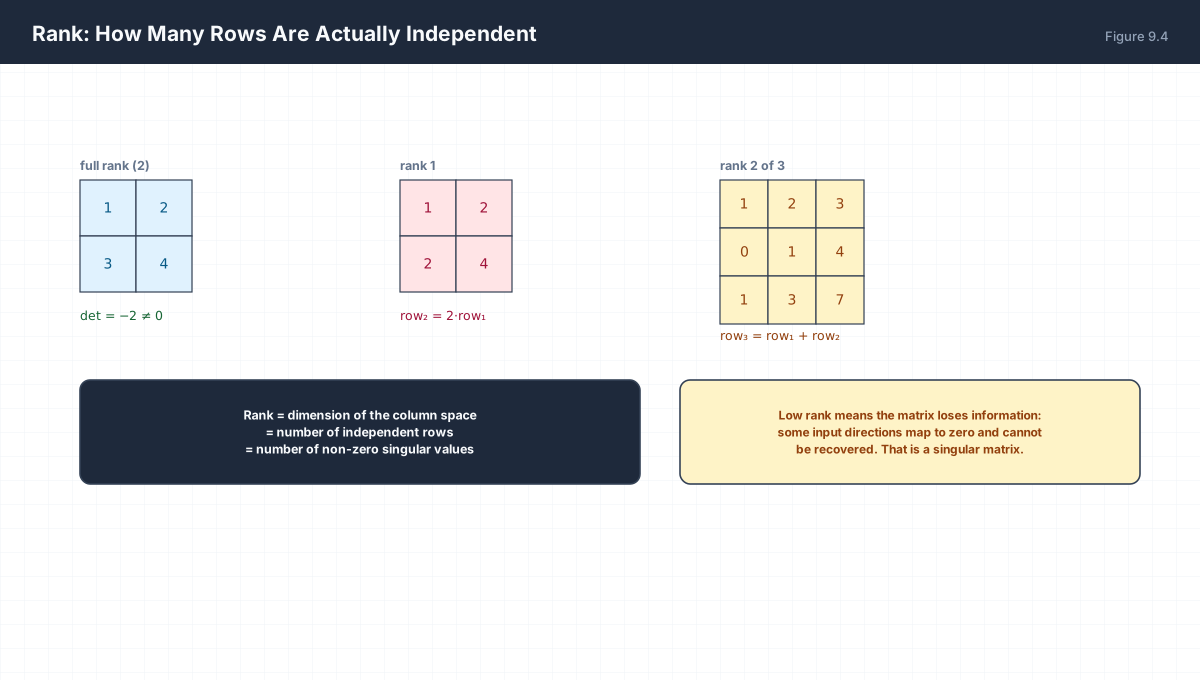
Rank is the dimension of the column space — equivalently the number of independent rows, equivalently the number of non-zero singular values. For an operator it answers one question: how many input directions survive?
import numpy as np

full = np.array([[1., 2.], [3., 4.]])
dep  = np.array([[1., 2.], [2., 4.]])
low  = np.array([[1., 2., 3.], [0., 1., 4.], [1., 3., 7.]])

for name, M in [("full", full), ("dependent", dep), ("rank-2", low)]:
    print(f"{name:10s} shape={M.shape} rank={np.linalg.matrix_rank(M)}")

# a deficient matrix has a non-trivial null space
print("null direction of dep:", np.linalg.svd(dep)[2][-1])
assert np.allclose(dep @ np.array([2., -1.]), 0.0)
A rank-deficient weight matrix has a null space: some non-zero input x maps to exactly zero output. That input is unrecoverable — the layer has destroyed it. This is the mathematics behind the observation that a low-rank projection discards information, and the reason LoRA’s low-rank updates are an approximation rather than a reparameterisation.
6. Data Versus Operator
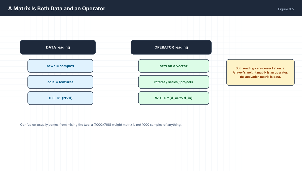
| Reading | Rows Mean | Shape Convention |
|---|---|---|
| Data | Samples | X ∈ ℝ^(N×d) — N samples, d features |
| Operator | Output dimensions | W ∈ ℝ^(d_out×d_in) — maps d_in → d_out |
The operator convention explains the shape of a weight matrix. A layer consuming x ∈ ℝ^(d_in) and producing y ∈ ℝ^(d_out) needs W such that Wx has d_out entries, so W is (d_out × d_in). This is the transpose of what many people expect from the “rows are samples” intuition, and it is exactly why PyTorch’s nn.Linear(in_features, out_features) stores weight as (out_features, in_features).
7. Worked Examples
7.1 Elementwise versus matrix product
A = [[1,2],[3,4]],  B = [[10,20],[30,40]]

A ⊙ B = [[10, 40], [90, 160]]        elementwise
A @ B = [[1·10+2·30, 1·20+2·40], [3·10+4·30, 3·20+4·40]]
      = [[70, 100], [150, 220]]      matrix product
7.2 Transpose of a product
X (2×3), Y (3×4)  →  XY is (2×4)
(XY)ᵀ is (4×2),  and  Yᵀ(3×4→4×3) @ Xᵀ(2×3→3×2) = (4×2)   ✓
7.3 Detect a rank deficiency
M = [[1,2],[2,4]]
row₂ = 2·row₁  →  rank 1
det(M) = 1·4 − 2·2 = 0  →  singular
null space: M @ (2,−1) = (0, 0)
7.4 Orthogonal matrix inverse is free
Q = rotation by 90° = [[0,−1],[1,0]]
Qᵀ = [[0,1],[−1,0]]
QᵀQ = I  →  Q⁻¹ = Qᵀ     no division required
7.5 Trace as a diagonal sum
tr(A) = Σᵢ A[i,i]
For A = [[1,2],[3,4]]:  tr = 1 + 4 = 5
8. Verify It in Python
import numpy as np

A = np.array([[1., 2.], [3., 4.]])
B = np.array([[10., 20.], [30., 40.]])

# --- 1. elementwise vs matrix product -----------------------------
assert np.allclose(A * B, [[10., 40.], [90., 160.]])
assert np.allclose(A @ B, [[70., 100.], [150., 220.]])
assert not np.allclose(A * B, A @ B)
print("Hadamard and matrix product differ as expected")

# --- 2. shapes and indexing ---------------------------------------
assert A.shape == (2, 2) and A.size == 4
assert np.allclose(A[0, :], [1., 2.]) and np.allclose(A[:, 1], [2., 4.])
print("row/column extraction ok")

# --- 3. transpose rules -------------------------------------------
M = np.random.rand(2, 3)
assert np.allclose(M.T.T, M)
X = np.random.rand(2, 3); Y = np.random.rand(3, 4)
assert np.allclose((X @ Y).T, Y.T @ X.T)
print("(AB)T = BT AT verified")

# --- 4. rank deficiency -------------------------------------------
dep = np.array([[1., 2.], [2., 4.]])
assert np.linalg.matrix_rank(dep) == 1
assert np.isclose(np.linalg.det(dep), 0.0)
assert np.allclose(dep @ np.array([2., -1.]), 0.0)     # null vector
print("rank-1 matrix has a null direction")

# --- 5. orthogonal inverse is the transpose ------------------------
Q = np.array([[0., -1.], [1., 0.]])
assert np.allclose(Q.T @ Q, np.eye(2))
assert np.allclose(np.linalg.inv(Q), Q.T)
print("Q^-1 == Q^T")

# --- 6. trace ------------------------------------------------------
assert np.isclose(np.trace(A), 5.0)
print("trace:", np.trace(A))

# --- 7. weight shape is (out, in) ---------------------------------
d_in, d_out = 768, 256
W = np.random.randn(d_out, d_in)
x = np.random.randn(d_in)
assert (W @ x).shape == (d_out,)
print("W(out,in) @ x(in) -> ", (W @ x).shape)
print("all assertions passed")
9. Practice Questions
- For
[[1,2,3],[4,5,6]], state the shape, extract row 1 and column 2, and give the size. - Compute both
A ⊙ BandA @ BforA=[[1,0],[0,1]]andB=[[2,3],[4,5]]. - Prove
(AB)ᵀ = BᵀAᵀusing index notation. - Give a 3×3 matrix with rank 2 and identify its null space.
- Why does
QᵀQ = IimplyQ⁻¹ = Qᵀ? - What shape is the weight matrix of a layer mapping 512 → 128, and why?
- What breaks if you use
*instead of@in a linear layer? - Is every diagonal matrix symmetric? Give a counterexample or prove it.
- Show that a rank-deficient weight matrix loses input information irrecoverably.
- Why does the residual connection
x + f(x)requirefto preserve shape?
10. Official References & Further Reading
Continue the Course
- Course Index: AI Mathematics Masterclass — All 48 Chapters
- Previous Chapter: Chapter 8: Vector Operations — Addition, Scaling, Norms & the Dot Product
- Next Chapter: Chapter 10: Matrix Multiplication & Linear Transformations
- Related Series: PyTorch Engineering Masterclass — All 16 Modules