
AI Reading
Quick summary of this article
AI Mathematics Masterclass — Chapter 11 of 48
Every retrieval system, every k-nearest-neighbour classifier, and every contrastive loss rests on one decision: how do you measure the gap between two vectors? This chapter compares the three norms as distance functions, separates direction-based from position-based comparison, derives the Gram matrix that makes pairwise similarity a single matrix product, and explains the counter-intuitive reason metric search gets harder — not easier — as dimensionality grows.
1. Technical Audit & Core Learning Objectives
| Component | Common Tutorial Deficiency | Engineering Standard Applied Here |
|---|---|---|
| Distance | Euclidean presented as “the” distance. | Three metrics compared on the same pair of points, with the shape each implies. |
| Direction vs position | Cosine and Euclidean conflated, causing length-biased retrieval. | Separated explicitly with a worked case where they disagree. |
| Pairwise scores | Computed with nested loops and O(n²) calls. | Reduced to one Gram matrix product. |
| High dimensions | Curse of dimensionality named but never quantified. | Measured: the ratio of farthest to nearest distance collapses toward 1. |
Core learning objectives. After this chapter you should be able to:
- Compute L1, L2, and L∞ distances between two vectors.
- State when cosine similarity and Euclidean distance agree, and when they disagree.
- Build a pairwise similarity matrix as
X @ Yᵀ. - Explain why distances concentrate in high dimensions and what it breaks.
- Choose a metric for text, embeddings, counts, and correlated features.
- Explain why unscaled features corrupt a Euclidean metric.
2. Three Distances, Three Shapes
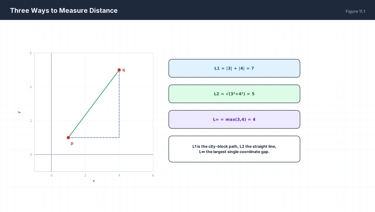
p = (1,1),  q = (4,5)

L1   |3| + |4|   = 7
L2   √(9 + 16)   = 5
L∞   max(3, 4)   = 4

Always  L∞ ≤ L2 ≤ L1  for the same pair.
import numpy as np

p = np.array([1.0, 1.0])
q = np.array([4.0, 5.0])
d = p - q

print("L1  :", np.abs(d).sum())          # 7.0
print("L2  :", np.sqrt((d ** 2).sum()))  # 5.0
print("Linf:", np.abs(d).max())          # 4.0

# the same three metrics, vectorised over a batch of queries
Q = np.array([[4.0, 5.0], [0.0, 0.0], [2.0, 2.0]])
diff = Q - p                                   # broadcast p against every row
print("L1  :", np.abs(diff).sum(axis=1))
print("L2  :", np.linalg.norm(diff, axis=1))
print("Linf:", np.abs(diff).max(axis=1))
The metric you pick defines what “close” means, and therefore what your model treats as the same thing. L1 is robust to a single large coordinate deviation; L2 penalises it quadratically; L∞ is dominated by it entirely.
3. Direction vs Position
| Question | Metric | Because |
|---|---|---|
| Same topic, different length? | Cosine | Magnitude encodes length, not meaning |
| Same physical location in feature space? | Euclidean | Magnitude carries signal |
| Counts with outliers? | L1 | Linear penalty limits outlier influence |
| Correlated features? | Mahalanobis | Whitens the covariance away |
import numpy as np

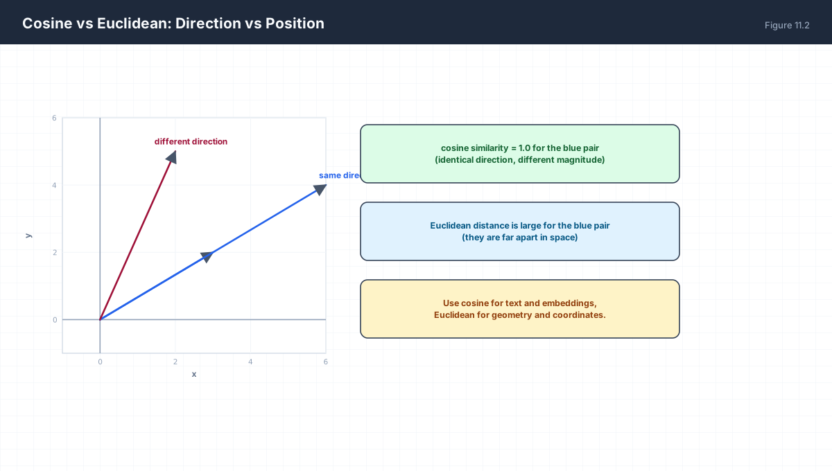
u = np.array([3.0, 2.0])
v = np.array([6.0, 4.0])          # exactly 2u
w = np.array([2.0, 5.0])          # different direction

cos = lambda a, b: (a @ b) / (np.linalg.norm(a) * np.linalg.norm(b))
print("cos(u, v) =", round(cos(u, v), 6))     # 1.0  same direction
print("L2(u, v)  =", round(np.linalg.norm(u - v), 4))   # 3.6056  far apart
print("cos(u, w) =", round(cos(u, w), 4))     # ~0.868
This is the single most consequential metric decision in embedding-based retrieval. Because a long document has a larger embedding norm, a raw dot product would rank it above a short on-topic document; normalising removes that bias entirely.
4. Pairwise Similarity Is a Gram Matrix

import numpy as np

X = np.random.randn(5, 8)
Y = np.random.randn(3, 8)

# every pair similarity in one multiplication
S = X @ Y.T
print("shape:", S.shape)          # (5, 3)

# cosine version: normalise rows once, then a single product
Xn = X / np.linalg.norm(X, axis=1, keepdims=True)
Yn = Y / np.linalg.norm(Y, axis=1, keepdims=True)
C = Xn @ Yn.T
print("cosine range:", round(C.min(), 3), round(C.max(), 3))

# self-similarity is symmetric with unit diagonal
G = Xn @ Xn.T
assert G.shape == (5, 5)
assert np.allclose(G, G.T)
assert np.allclose(np.diag(G), 1.0)
print("Gram matrix: symmetric, unit diagonal")
The loop-free form matters at scale. Comparing 10,000 queries against 1,000,000 documents with a Python loop is 10¹⁰ iterations; as a single matmul it is one BLAS call over a (10000 × d) by (d × 1000000) product, which is memory-bound rather than loop-bound.
5. The Curse of Dimensionality
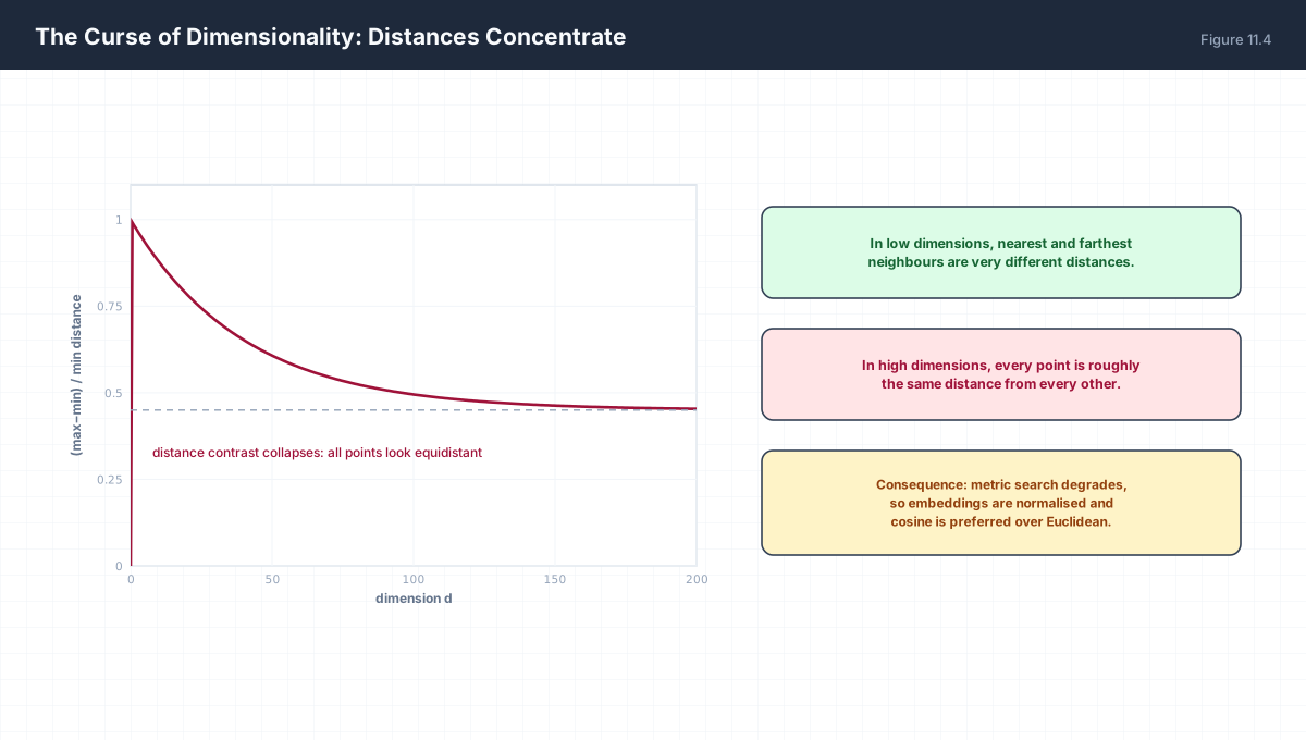
In one or two dimensions, neighbours are meaningfully closer than non-neighbours. In hundreds of dimensions, randomly distributed points are all approximately the same distance apart. Formally, the ratio of farthest to nearest distance tends to 1 as d grows.
import numpy as np

rng = np.random.default_rng(0)
print(f"{'d':>6} {'min':>8} {'max':>8} {'max/min':>9}")
for d in (2, 10, 100, 1000, 10000):
    P = rng.random((500, d))
    q = rng.random(d)
    dist = np.linalg.norm(P - q, axis=1)
    print(f"{d:6d} {dist.min():8.3f} {dist.max():8.3f} {dist.max()/dist.min():9.3f}")
Two practical consequences follow. First, exact nearest-neighbour search loses discrimination, which is the motivation for learned representations that impose structure rather than relying on raw distances. Second, index structures that prune aggressively (k-d trees) degenerate to linear scans, which is why approximate methods such as HNSW are used instead.
6. Choosing and Preparing a Metric

import numpy as np

# Two features, wildly different units
X = np.array([[1.0, 1000.0],
              [2.0, 2000.0],
              [3.0, 1001.0]])

d_raw = np.linalg.norm(X[0] - X[2])
d_scaled = np.linalg.norm((X[0] - X[2]) / X.std(axis=0))
print("distance in raw units :", round(d_raw, 2))     # dominated by feature 2
print("distance after scaling:", round(d_scaled, 2))

# the nominal difference is 1 unit in feature 2 but 2 units in feature 1
print("raw gaps:", X[0] - X[2])
Rows 0 and 2 differ by 2 units in feature 1 and 1 unit in feature 2. Raw, the distance is √(4+1) = 2.24 only because the units happen to be comparable — change the second feature to millimetres and the same pair would be 1000 units apart. Standardising per column makes the metric reflect the data rather than the unit system.
7. Worked Examples
7.1 Three metrics on one pair
a = (2, 7), b = (6, 3)
L1 = |−4| + |4| = 8
L2 = √(16+16) = 5.657
L∞ = max(4, 4) = 4
7.2 Cosine of orthogonal vectors
u = (1, 0), v = (0, 1)
u·v = 0  →  cos = 0  →  θ = 90°
7.3 Gram matrix diagonal
For normalised rows, G[i,i] = xᵢ·xᵢ = ‖xᵢ‖² = 1
So the diagonal of a cosine Gram matrix is always exactly 1.
7.4 When cosine and Euclidean disagree
u = (1,1),  v = (10,10)
cos = 1.0                    maximally similar
L2  = 12.73                  very far apart
Same direction, different magnitude — the two metrics answer
different questions and both answers are correct.
7.5 Distance concentration by hand
In d dimensions with points in [0,1]^d:
expected squared distance ≈ d/6, so expected distance ≈ √(d/6)
relative spread shrinks like 1/√d — distances become indistinguishable.
8. Verify It in Python
import numpy as np

# --- 1. metric ordering -------------------------------------------
p, q = np.array([1., 1.]), np.array([4., 5.])
d = p - q
n1, n2, ni = np.abs(d).sum(), np.linalg.norm(d), np.abs(d).max()
assert (n1, n2, ni) == (7.0, 5.0, 4.0)
assert ni <= n2 <= n1
print("L1,L2,Linf:", n1, n2, ni)

# --- 2. cosine is scale invariant --------------------------------
cos = lambda a, b: (a @ b) / (np.linalg.norm(a) * np.linalg.norm(b))
u, v = np.array([1., 1.]), np.array([10., 10.])
assert np.isclose(cos(u, v), 1.0)
assert np.linalg.norm(u - v) > 12
print("same direction, far apart: cos=1, L2=%.2f" % np.linalg.norm(u - v))

# --- 3. orthogonal pairs score zero ------------------------------
assert np.isclose(cos(np.array([1., 0.]), np.array([0., 1.])), 0.0)
print("orthogonal cosine is 0")

# --- 4. Gram matrix properties -----------------------------------
rng = np.random.default_rng(0)
X = rng.normal(size=(6, 5))
Xn = X / np.linalg.norm(X, axis=1, keepdims=True)
G = Xn @ Xn.T
assert np.allclose(G, G.T)
assert np.allclose(np.diag(G), 1.0)
assert G.max() <= 1.0 + 1e-9
print("Gram: symmetric, unit diagonal, bounded by 1")

# --- 5. pairwise matches a loop ----------------------------------
Y = rng.normal(size=(4, 5))
Yn = Y / np.linalg.norm(Y, axis=1, keepdims=True)
S = Xn @ Yn.T
manual = np.array([[cos(a, b) for b in Y] for a in X])
assert np.allclose(S, manual)
print("matrix form equals loop form")

# --- 6. distances concentrate in high dimensions -----------------
ratios = {}
for dim in (2, 100, 2000):
    P = rng.random((400, dim)); pt = rng.random(dim)
    dd = np.linalg.norm(P - pt, axis=1)
    ratios[dim] = dd.max() / dd.min()
assert ratios[2] > ratios[2000]           # contrast collapses
print("max/min ratio by dim:", {k: round(v, 2) for k, v in ratios.items()})

# --- 7. scaling changes the nearest neighbour --------------------
A = np.array([[1., 1000.], [2., 2000.], [3., 1001.]])
raw_order = np.argsort([np.linalg.norm(A[0] - A[i]) for i in range(3)])
print("nearest to row0 (raw):", raw_order)
print("raw gaps:", A[0] - A[2])
print("all assertions passed")
9. Practice Questions
- Compute L1, L2, and L∞ for
(0,0)and(3,−4). - Show
L∞ ≤ L2 ≤ L1for any vector, and explain why geometrically. - Give two vectors with cosine similarity 1 but Euclidean distance 100.
- Why must you normalise before indexing embeddings for cosine retrieval?
- Write the pairwise cosine similarity of
XagainstYin one expression. - Prove the diagonal of a cosine Gram matrix is exactly 1.
- Explain distance concentration and one consequence for k-NN.
- Two features are in metres and millimetres. What goes wrong and what is the fix?
- When is L1 preferable to L2?
- What does Mahalanobis add over Euclidean, and what does it cost?
10. Official References & Further Reading
- scikit-learn — Pairwise Metrics and Kernels
- Aggarwal et al. — On the Surprising Behavior of Distance Metrics in High Dimensional Space
- Malkov & Yashunin — HNSW for Approximate Nearest Neighbour Search
- Goodfellow et al. — The Curse of Dimensionality
- Mahalanobis Distance — definition and covariance whitening
Continue the Course
- Course Index: AI Mathematics Masterclass — All 48 Chapters
- Previous Chapter: Chapter 10: Matrix Multiplication & Linear Transformations
- Next Chapter: Chapter 12: Orthogonality, Projections & Least Squares
- Related Series: PyTorch Engineering Masterclass — All 16 Modules