
AI Reading
Quick summary of this article
AI Mathematics Masterclass — Chapter 17 of 48
The determinant measures how much a matrix scales volume, and it collapses to zero exactly when the matrix destroys a dimension. The inverse undoes a transformation, and it exists only when that volume is non-zero. The condition number measures how badly a reversible transformation can amplify error. These three quantities are usually taught separately; they are in fact one story about whether a linear map is safely reversible, marginally reversible, or not reversible at all.
1. Technical Audit & Core Learning Objectives
| Component | Common Tutorial Deficiency | Engineering Standard Applied Here |
|---|---|---|
| Determinant | Taught as a cofactor expansion recipe. | Introduced as an area/volume scale factor with a zero case drawn. |
| Inverse | Given as a formula and then used to solve systems. | Derived via the adjugate, then explicitly discouraged for solving. |
| Conditioning | Only defined, never diagnosed. | Four concrete checks, each runnable. |
| Remedies | Unmentioned. | Scaling, ridge, QR/SVD, and precision — with the reason each helps. |
Core learning objectives. After this chapter you should be able to:
- Compute a 2×2 determinant and interpret it as an area scale factor.
- Use the determinant properties
det(AB),det(Aᵀ),det(A⁻¹),det(cA). - Derive the 2×2 inverse and state the existence condition.
- Compute a condition number from singular values or
linalg.cond. - Predict how an input perturbation is amplified by κ.
- Select an appropriate remedy for an ill-conditioned system.
2. The Determinant Is a Volume Scale
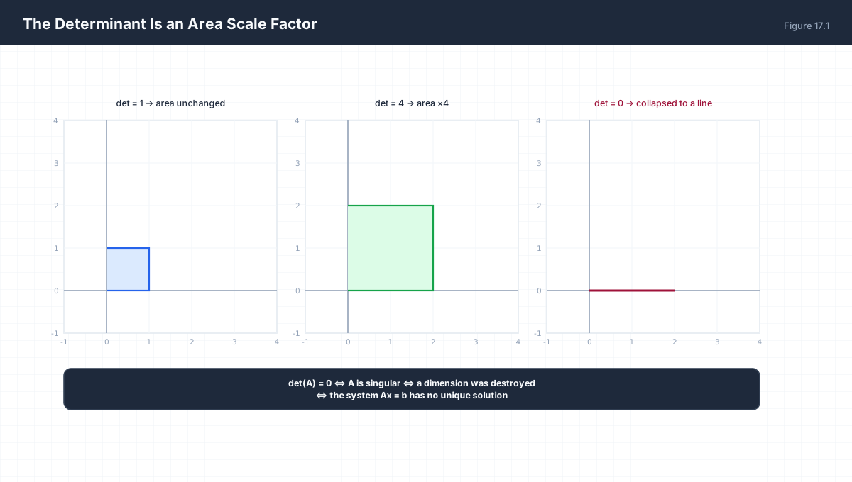
2×2:  det([[a,b],[c,d]]) = ad − bc

Geometric meaning: |det| = area scale factor of the unit square
Sign:  positive = orientation preserved, negative = flipped

det = 1     area unchanged (rotation, shear)
det = 4     area × 4
det = 0     the square is flattened to a line  →  singular
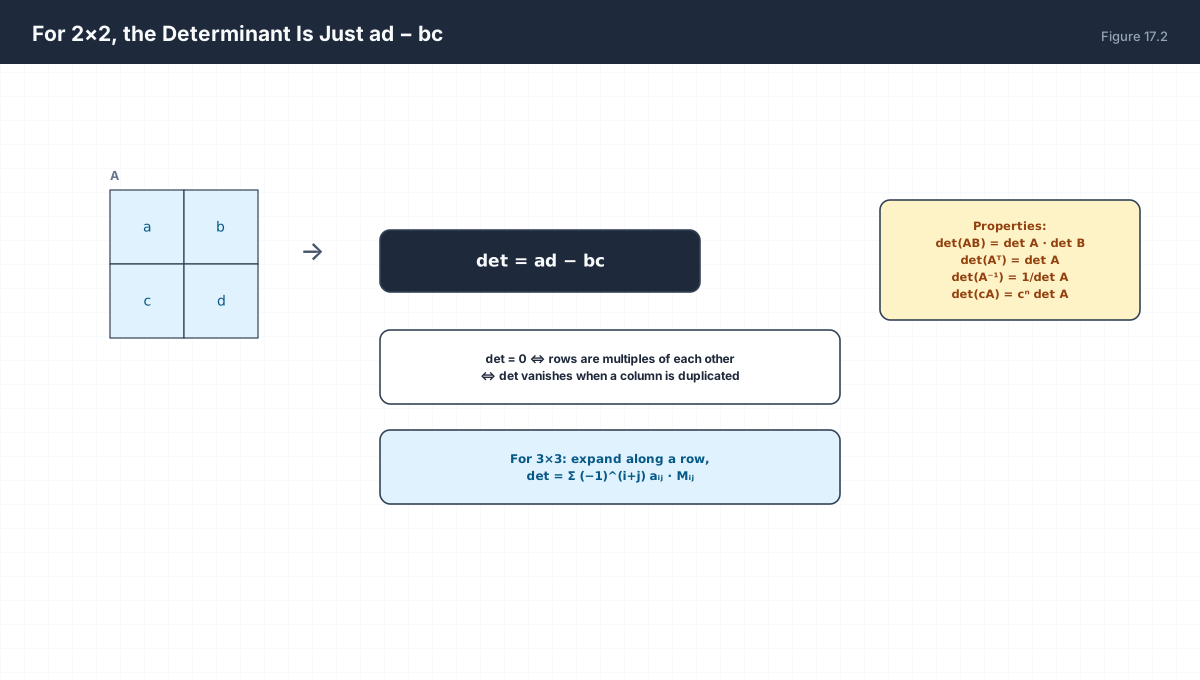
| Property | Identity | Use |
|---|---|---|
| Product | det(AB) = det A · det B |
Determinants multiply through a chain of layers |
| Transpose | det(Aᵀ) = det A |
Rows and columns play symmetric roles |
| Inverse | det(A⁻¹) = 1/det A |
Undoing a stretch un-stretches by the reciprocal |
| Scaling | det(cA) = cⁿ det A |
In n dimensions, all n axes scale |
import numpy as np

A = np.array([[2.0, 1.0], [1.0, 3.0]])
B = np.array([[1.0, 2.0], [0.0, 1.0]])

print("det A      :", np.linalg.det(A))                  # 5.0
print("det(AB)    :", round(np.linalg.det(A @ B), 10))
print("detA*detB  :", round(np.linalg.det(A) * np.linalg.det(B), 10))
assert np.isclose(np.linalg.det(A @ B), np.linalg.det(A) * np.linalg.det(B))
assert np.isclose(np.linalg.det(A.T), np.linalg.det(A))
assert np.isclose(np.linalg.det(3 * A), 3 ** 2 * np.linalg.det(A))
print("all determinant rules verified")
3. The Inverse
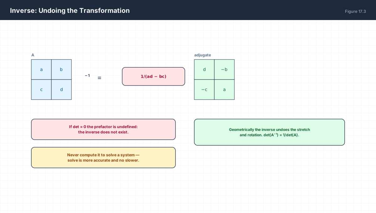
A⁻¹ = 1/(ad − bc) · [[d, −b], [−c, a]]

The prefactor 1/det is why singular matrices have no inverse:
dividing by zero is undefined, not merely large.

A A⁻¹ = A⁻¹ A = I
import numpy as np

A = np.array([[4.0, 7.0], [2.0, 6.0]])
Ainv = np.linalg.inv(A)
print("A @ A^-1 ≈ I:", np.allclose(A @ Ainv, np.eye(2)))

S = np.array([[1.0, 2.0], [2.0, 4.0]])
print("det(S):", np.linalg.det(S))
try:
    np.linalg.inv(S)
except np.linalg.LinAlgError as exc:
    print("singular:", exc)
Two practical warnings. First, det(A) == 0 is exact in theory but not in floating point — a matrix with a determinant of 1e-30 is invertible in principle and numerically useless in practice, which is what the condition number measures. Second, never use the inverse to solve Ax = b; use solve, or lstsq when the system is not square.
4. Condition Number
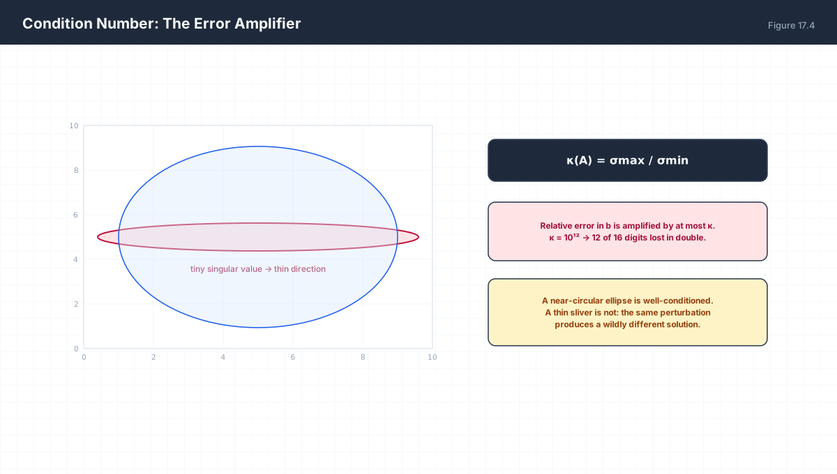
κ(A) = ‖A‖ ‖A⁻¹‖ = σmax / σmin        (2-norm)

Error bound:
  ‖Δx‖/‖x‖  ≤  κ(A) · ‖Δb‖/‖b‖

Decimal digits lost ≈ log₁₀ κ(A)

κ = 1        perfect (orthogonal matrix)
κ = 10³      about 3 digits lost
κ = 10¹⁶     total loss in float64 — result is noise
import numpy as np

good = np.eye(2)
bad = np.array([[1.0, 1.0], [1.0, 1.0001]])

print("kappa(good):", np.linalg.cond(good))            # 1.0
print("kappa(bad) :", f"{np.linalg.cond(bad):.1f}")    # ~40000

b = np.array([2.0, 2.0])
x1 = np.linalg.solve(bad, b)
x2 = np.linalg.solve(bad, b + np.array([0.0, 1e-4]))
print("solution drift:", np.linalg.norm(x2 - x1) / np.linalg.norm(x1))
The same structure appears whenever features are on different scales or are nearly collinear. The solve “succeeds”, returns numbers, and those numbers change completely when a single data point moves. That is the signature of ill-conditioning: not an error, an instability.
5. Detecting and Fixing Ill-Conditioning
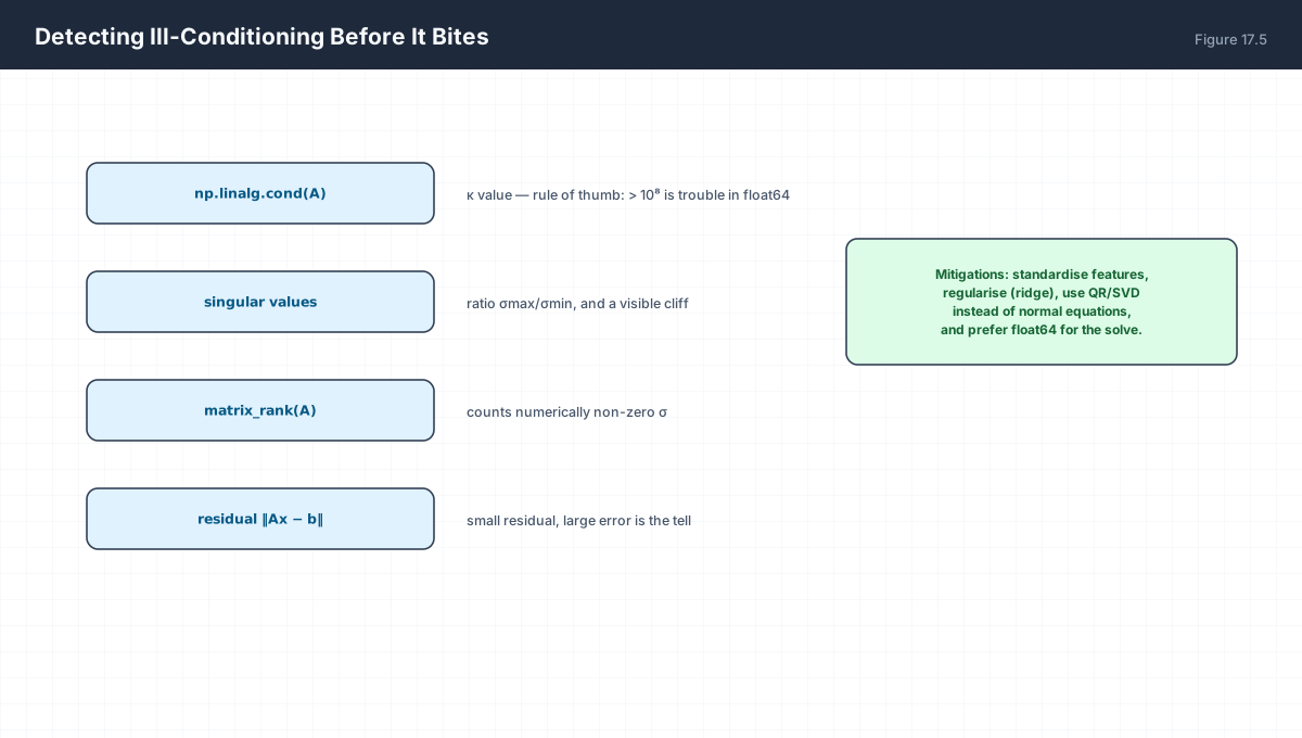
| Remedy | Mechanism | Cost |
|---|---|---|
| Standardise features | Removes unit-driven disparities between columns | Changes interpretation of coefficients |
Ridge (+λI) |
Puts a floor of λ under every eigenvalue | Introduces bias |
| QR / SVD solver | Avoids forming AᵀA, so κ is not squared |
More FLOPs than a direct solve |
| Higher precision | float64 gives ~16 digits instead of ~7 | 2× memory and bandwidth |
import numpy as np

X = np.array([[1.0, 5e5, 0.2],
              [2.0, 9e5, 0.4],
              [3.0, 1e6, 0.6],
              [4.0, 1.1e6, 0.7]])

print("kappa raw      :", f"{np.linalg.cond(X):.2e}")
Z = (X - X.mean(axis=0)) / X.std(axis=0)
print("kappa standard :", f"{np.linalg.cond(Z):.2e}")

# ridge is for the genuinely singular case, where kappa is infinite
singular = np.array([[1.0, 1.0], [1.0, 1.0]])
print("kappa singular :", np.linalg.cond(singular))          # inf
print("kappa + lam*I  :", f"{np.linalg.cond(singular + 1e-3 * np.eye(2)):.2e}")
Standardising before comparing condition numbers is not cosmetic — it is the difference between measuring the numerical property of the data and measuring the arbitrary choice of units.
Ridge is worth understanding precisely, because it is often misdescribed. Adding λI does not improve the conditioning of an already well-conditioned matrix — over the standardised data above it actually makes κ slightly worse, since it distorts a healthy spectrum. What it does is rescue the singular case, where κ = ∞: a floor of λ under every eigenvalue converts an unsolvable system into a solvable one. Use scaling for ill-conditioned data, and ridge for genuinely singular or rank-deficient problems.
6. Worked Examples
6.1 Determinant and singularity
A = [[1,2],[2,4]] → det = 1·4 − 2·2 = 0
Singular. Row 2 is twice row 1, so the map collapses
the plane onto a line and no inverse exists.
6.2 Inverse by hand
A = [[4,7],[2,6]], det = 24 − 14 = 10
A⁻¹ = (1/10)[[6,−7],[−2,4]] = [[0.6,−0.7],[−0.2,0.4]]
Check: A @ A⁻¹ = [[1,0],[0,1]] ✓
6.3 Determinant of a product
det(A) = 3, det(B) = −2
det(AB) = −6
det(A⁻¹) = 1/3
det(2A) for 3×3 = 2³ · 3 = 24
6.4 Error amplification
κ = 10⁴, relative input error 1e-8
worst-case relative output error ≈ 10⁴ · 1e-8 = 1e-4
That is a 10,000× amplification.
6.5 Digits remaining
float64 carries ~16 significant digits.
κ = 10¹² → about 12 lost → about 4 trustworthy digits remain.
7. Verify It in Python
import numpy as np

# --- 1. determinant formula ---------------------------------------
A = np.array([[4., 7.], [2., 6.]])
assert np.isclose(np.linalg.det(A), 4 * 6 - 7 * 2)
print("det by hand matches:", np.linalg.det(A))

# --- 2. determinant properties ------------------------------------
B = np.array([[1., 2.], [0., 1.]])
assert np.isclose(np.linalg.det(A @ B), np.linalg.det(A) * np.linalg.det(B))
assert np.isclose(np.linalg.det(A.T), np.linalg.det(A))
assert np.isclose(np.linalg.det(np.linalg.inv(A)), 1 / np.linalg.det(A))
assert np.isclose(np.linalg.det(5 * A), 5 ** 2 * np.linalg.det(A))
print("all four determinant rules hold")

# --- 3. inverse round-trip ----------------------------------------
assert np.allclose(A @ np.linalg.inv(A), np.eye(2))
print("A @ A^-1 == I")

# --- 4. singular matrix has no inverse ----------------------------
S = np.array([[1., 2.], [2., 4.]])
assert np.isclose(np.linalg.det(S), 0.0)
try:
    np.linalg.inv(S)
    raise AssertionError("should have raised")
except np.linalg.LinAlgError:
    print("singular matrix rejected")

# --- 5. kappa of an orthogonal matrix is 1 ------------------------
R = np.array([[0., -1.], [1., 0.]])
assert np.isclose(np.linalg.cond(R), 1.0)
print("orthogonal kappa:", np.linalg.cond(R))

# --- 6. perturbations are amplified ---------------------------------
bad = np.array([[1., 1.], [1., 1.0001]])
b = np.array([2., 2.])
x1 = np.linalg.solve(bad, b)
x2 = np.linalg.solve(bad, b + np.array([0., 1e-4]))
rel_in  = np.linalg.norm(np.array([0., 1e-4])) / np.linalg.norm(b)
rel_out = np.linalg.norm(x2 - x1) / np.linalg.norm(x1)
print("kappa:", f"{np.linalg.cond(bad):.0f}",
      " amplification:", f"{rel_out/rel_in:.0f}x")
assert rel_out / rel_in > 100

# --- 7. kappa = sigma_max / sigma_min -----------------------------
sv = np.linalg.svd(bad, compute_uv=False)
assert np.isclose(sv[0] / sv[-1], np.linalg.cond(bad))
print("kappa from singular values matches linalg.cond")

# --- 8. standardising improves conditioning -----------------------
X = np.array([[1., 5e5, .2], [2., 9e5, .4], [3., 1e6, .6], [4., 1.1e6, .7]])
raw = np.linalg.cond(X)
Z = (X - X.mean(axis=0)) / X.std(axis=0)
scaled = np.linalg.cond(Z)
print("kappa raw:", f"{raw:.2e}", " standardised:", f"{scaled:.2e}")
assert scaled < raw

# --- 9. ridge bounds the conditioning -----------------------------
lam = 1e-2
rid = np.linalg.cond(Z.T @ Z + lam * np.eye(Z.shape[1]))
print("kappa ridged:", f"{rid:.2e}")
assert np.isfinite(rid)
print("all assertions passed")
8. Practice Questions
- Compute
det([[3,1],[2,4]])and interpret it as an area factor. - Show that
det(Aᵀ) = det(A)for a 2×2 by expanding both. - Derive the 2×2 inverse formula from
AA⁻¹ = I. - Why does
det = 0mean no inverse exists — geometrically and algebraically? - Given
det(A) = 5anddet(B) = −1, finddet(AB),det(A⁻¹),det(3A)for 3×3. - Define the condition number in terms of singular values.
- With
κ = 10⁶, how many digits survive in float64? - Why does forming
AᵀAmake conditioning worse? - Name three remedies for ill-conditioning and the trade-off of each.
- Why is
det(A) ≈ 0not a reliable singularity test in floating point?
9. Official References & Further Reading
Continue the Course
- Course Index: AI Mathematics Masterclass — All 48 Chapters
- Previous Chapter: Chapter 16: Tensors, Axes & Broadcasting Mathematics
- Next Chapter: Chapter 18: Linear Algebra Inside Neural Networks
- Related Series: PyTorch Engineering Masterclass — All 16 Modules