
AI Reading
Quick summary of this article
AI Mathematics Masterclass — Chapter 5 of 48
Every loss function is a sum. Every batch reduction is a sum. Attention is a weighted sum, convolution is a sliding sum of products, and a joint probability over a sequence is a product that becomes a sum in log space. This chapter makes summation notation fully operational: how to read a Σ with its indices, how each Σ consumes exactly one axis, when an infinite series is allowed to be rearranged, and how Einstein notation compresses the whole vocabulary into a single operator.
1. Technical Audit & Core Learning Objectives
Summation is usually taught as a notation shorthand and then never used again, leaving a gap where the practitioner can write a training loop but cannot read the loss definition in a paper.
| Component | Common Tutorial Deficiency | Engineering Standard Applied Here |
|---|---|---|
| Anatomy | Start index, end index, and body shown once, then assumed obvious. | Each part named and mapped to its array equivalent in the same breath. |
| Nested sums | Presented as algebra, with the rank bookkeeping left implicit. | “One Σ removes one axis” used as the primary reading rule. |
| Convergence | Infinite series treated as a curiosity. | Rearrangement validity tied to absolute convergence, which is why batch accumulators are safe. |
| Einstein notation | Omitted, leaving einsum unreadable. |
Taught as the general form of which matmul and dot product are special cases. |
Core learning objectives. After this chapter you should be able to:
- Expand
Σᵢ₌₁ⁿ f(i)by hand and translate it to a vectorised reduction. - Predict the output rank of a nested sum by counting Σ signs.
- Distinguish a sequence, a series, and a partial sum.
- State the divergence test and use it to rule out convergence.
- Write a convolution, a weighted average, and a dot product as summations.
- Read and write
einsumstrings for multi-axis contractions.
2. Anatomy of a Summation
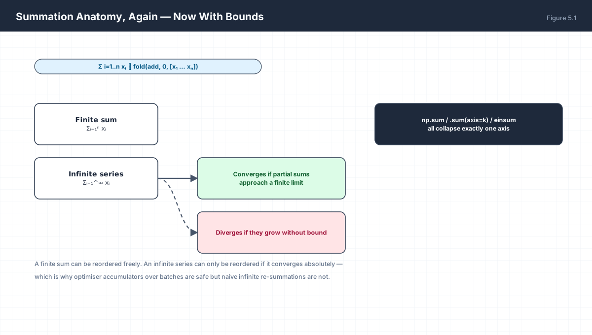
  n
  Σ  xᵢ  =  x₁ + x₂ + x₃ + … + xₙ
 i=1
| Part | Meaning | Array Equivalent |
|---|---|---|
Σ |
Add the terms | .sum() |
i = 1 |
Where the index starts | array[1:] if 1-based |
n |
Where it stops (inclusive) | the axis length |
xᵢ |
The term, as a function of the index | the array being reduced |
Three collapse rules follow immediately and are worth memorising:
Σᵢ₌₁ⁿ c        = n·c              a constant summed n times
Σᵢ₌₁ⁿ c·xᵢ     = c·Σᵢ₌₁ⁿ xᵢ       constants factor out
Σᵢ₌₁ⁿ (xᵢ + yᵢ) = Σxᵢ + Σyᵢ       sums distribute over addition
3. Nested Sums and the One-Axis Rule
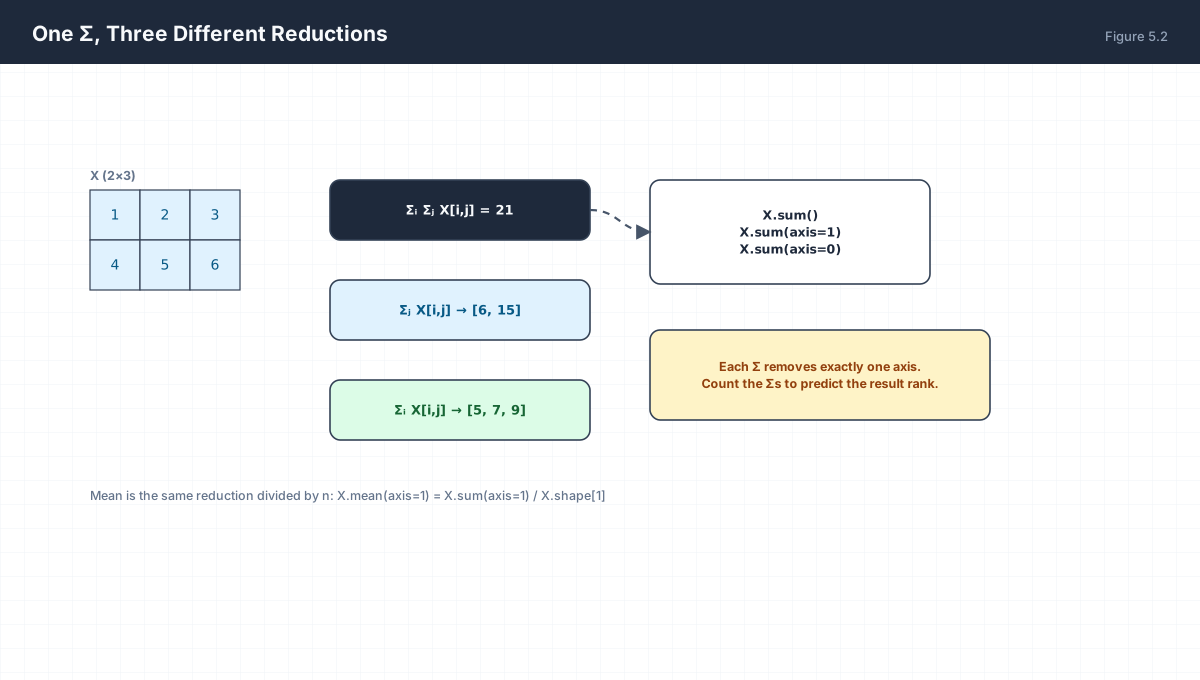
A double sum such as Σᵢ Σⱼ A[i,j] reduces a matrix to a scalar. Each Σ removes exactly one axis, so the rank of the result equals the rank of the operand minus the number of summation signs.
import numpy as np

X = np.array([[1.0, 2.0, 3.0],
              [4.0, 5.0, 6.0]])

print("Σᵢ Σⱼ X[i,j] :", X.sum())            # 21.0   scalar
print("Σⱼ X[i,j]     :", X.sum(axis=1))      # [6. 15.]  one value per row
print("Σᵢ X[i,j]     :", X.sum(axis=0))      # [5. 7. 9.] one value per column
print("mean          :", X.mean(axis=1))     # [2. 5.]  sum / 3
Note the correspondence carefully, because it trips people up constantly: Σⱼ means “sum over the column index”, so the column axis disappears and one number remains per row. The surviving index becomes the output’s axis, and axis= in NumPy names the axis being removed, not the one being kept.
3.1 Upper-triangle sums
Σᵢ₌₁ⁿ Σⱼ₌ᵢⁿ A[i,j]     the upper triangle, including the diagonal

For n = 3 this is A[1,1]+A[1,2]+A[1,3] + A[2,2]+A[2,3] + A[3,3]
i.e. six terms, not nine.  In NumPy:  np.triu(A).sum()
4. Sequences, Series, and Partial Sums
Three terms are often conflated:
- Sequence — an ordered list:
a₁, a₂, a₃, … - Series — the sum of a sequence:
Σ aᵢ - Partial sum — the sum of the first
nterms:Sₙ = Σᵢ₌₁ⁿ aᵢ
| Series | Converges? | Limit |
|---|---|---|
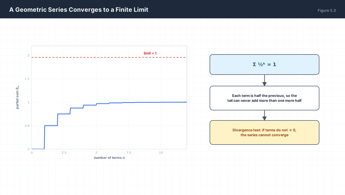
Σ ½ᵏ |
Yes | 1 |
Σ 1/k² |
Yes | π²/6 ≈ 1.6449 |
Σ 1/k |
No | diverges (harmonic) |
Σ (−1)ᵏ |
No | terms do not tend to 0 |
The divergence test is the cheapest check available: if the terms aᵢ do not approach zero, the series cannot converge. It is necessary but not sufficient — the harmonic series has terms going to zero and still diverges, which is why Σ1/k is the standard counterexample.
The machine-learning relevance is the rearrangement question. A finite sum may be reordered freely. An infinite series may only be reordered if it converges absolutely; the alternating harmonic series converges, but reordering it can produce any value you like. In practice, every sum you compute over a batch is finite, so accumulation order is safe to change — which is exactly what lets a vectorised reduction be faster than a Python loop without changing the answer.
5. Weighted Sums and Attention
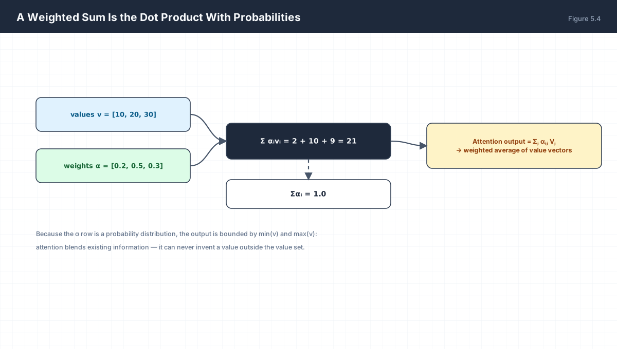
The most important summation in modern deep learning is a weighted sum whose weights form a probability distribution.
import numpy as np

values  = np.array([10.0, 20.0, 30.0])
weights = np.array([0.2, 0.5, 0.3])

assert np.isclose(weights.sum(), 1.0)
out = np.sum(weights * values)          # Σ αᵢvᵢ
print("weighted sum:", out)             # 21.0
print("bounded by values:", values.min() <= out <= values.max())

# batched: 4 queries x 3 keys, one distribution per query
alpha = np.array([[0.2, 0.5, 0.3],
                  [0.0, 1.0, 0.0],
                  [0.5, 0.5, 0.0],
                  [0.1, 0.1, 0.8]])
assert np.allclose(alpha.sum(axis=1), 1.0)
print("attention output:", alpha @ values)   # [21. 20. 15. 27.]
Two structural facts follow from the weights summing to one. First, the output is a convex combination: it cannot exceed the range of the values, so attention blends existing information rather than inventing new magnitudes. Second, if one weight is 1.0 the others must be 0.0, which is the mathematical description of a hard lookup — exactly what happens when an attention head becomes fully confident.
6. Convolution as a Sliding Sum
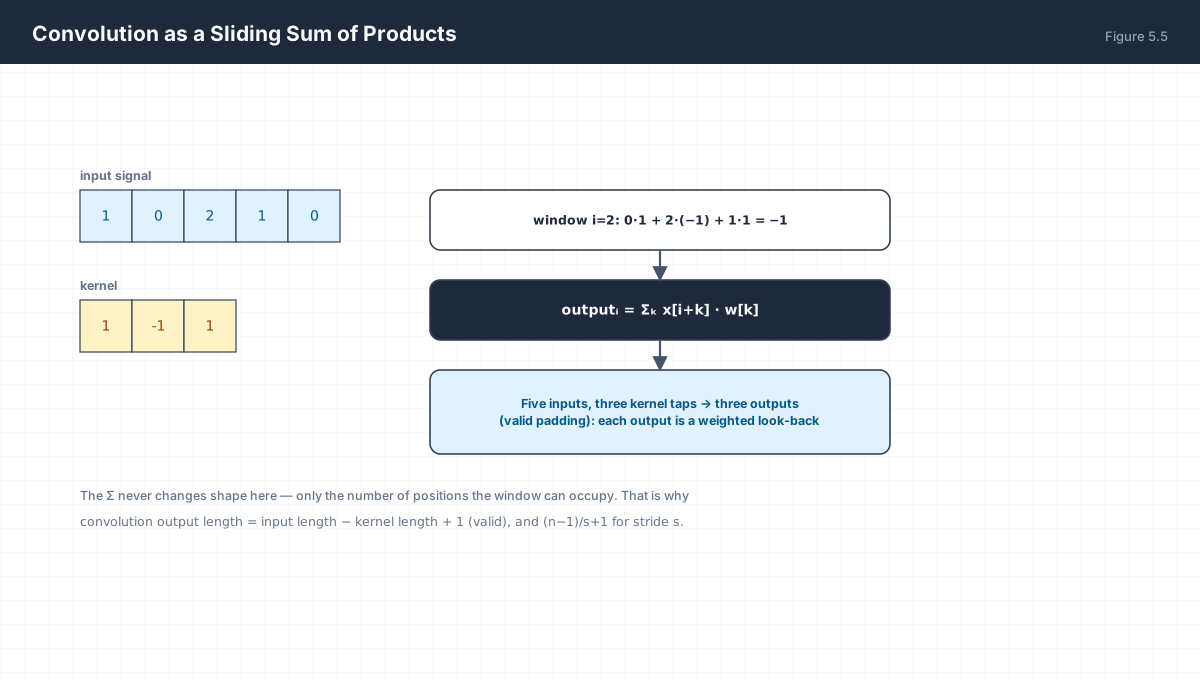
import numpy as np

def conv1d_valid(x, w):
    """out[i] = Σ_k x[i+k] * w[k]  -- valid padding, stride 1."""
    n, k = len(x), len(w)
    return np.array([np.sum(x[i:i + k] * w) for i in range(n - k + 1)])

x = np.array([1.0, 0.0, 2.0, 1.0, 0.0])
w = np.array([1.0, -1.0, 1.0])

out = conv1d_valid(x, w)
print("output:", out)                  # [3. -1. 1.]  (n - k + 1 = 3 positions)
assert len(out) == len(x) - len(w) + 1
print("manual first term: 1*1 + 0*(-1) + 2*1 =", 1*1 + 0*(-1) + 2*1)
The output length formula n − k + 1 for valid padding, and (n − k)/s + 1 for stride s, follows directly from counting how many positions the window can occupy. Nothing about the Σ changes between a convolution and a dot product — only which elements are multiplied together.
7. Einstein Summation
Einstein notation removes the Σ entirely: any index appearing exactly twice in a term is summed over implicitly. This makes every contraction a single expression and makes einsum the most general array operator available.
| Expression | Summation Form | einsum |
|---|---|---|
| dot product | Σᵢ aᵢbᵢ |
'i,i->' |
| matrix-vector | Σⱼ A[i,j]xⱼ |
'ij,j->i' |
| matrix product | Σⱼ A[i,j]B[j,k] |
'ij,jk->ik' |
| outer product | aᵢbⱼ (no sum) |
'i,j->ij' |
| trace | Σᵢ A[i,i] |
'ii->' |
| attention scores | Σ_d Q[b,h,i,d]K[b,h,j,d] |
'bhid,bhjd->bhij' |
import numpy as np

A = np.random.rand(3, 4)
B = np.random.rand(4, 5)

ref = A @ B
eins = np.einsum('ij,jk->ik', A, B)
print("matmul matches einsum:", np.allclose(ref, eins))

x = np.random.rand(4)
print("matvec matches:", np.allclose(A @ x, np.einsum('ij,j->i', A, x)))

S = np.random.rand(4, 4)
print("trace matches :", np.isclose(np.trace(S), np.einsum('ii->', S)))
8. Worked Examples
8.1 Expand and evaluate
Compute Σᵢ₌₁⁴ (3i − 1).
i=1: 2   i=2: 5   i=3: 8   i=4: 11
Σ = 2 + 5 + 8 + 11 = 26
Check with the linearity rule: 3·Σi − Σ1 = 3(10) − 4 = 26 ✓
8.2 Double sum by hand
Compute Σᵢ₌₁³ Σⱼ₌₁² (i·j).
i=1: 1·1 + 1·2 = 3
i=2: 2·1 + 2·2 = 6
i=3: 3·1 + 3·2 = 9
Σ = 18

Shortcut: (Σi)(Σj) = (1+2+3)(1+2) = 6·3 = 18  -- separable indices factor out
8.3 Mean is a scaled sum
Express the mean of n numbers as a summation and as an array call.
x̄ = (1/n) Σᵢ₌₁ⁿ xᵢ → x.mean() or x.sum() / len(x)
8.4 Geometric series partial sum
Compute the first five partial sums of Σ (1/3)ᵏ for k ≥ 1 and state the limit.
S = 1/3 + 1/9 + 1/27 + 1/81 + 1/243
  = 0.3333 + 0.1111 + 0.0370 + 0.0123 + 0.0041 = 0.4980

Limit for |r| < 1:  a/(1−r) = (1/3)/(1 − 1/3) = 0.5
8.5 Predict the rank
Given a rank-4 tensor T[b,h,i,d], what is the rank of Σ_d T?
One Σ over d → rank 3, shape (b, h, i)
9. Verify It in Python
import numpy as np

# --- 1. Linearity rules hold ---------------------------------------
xs = np.array([2.0, 5.0, 8.0, 11.0])
assert np.isclose(xs.sum(), 3 * np.arange(1, 5).sum() - 4)
print("Σ(3i-1) =", xs.sum())                       # 26.0

# --- 2. One Σ removes one axis -------------------------------------
T = np.arange(2 * 3 * 4 * 5, dtype=float).reshape(2, 3, 4, 5)
assert T.sum(axis=3).shape == (2, 3, 4)
assert T.sum(axis=(2, 3)).shape == (2, 3)
print("rank after Σ_d:", T.sum(axis=3).shape)
print("rank after Σ_i Σ_d:", T.sum(axis=(2, 3)).shape)

# --- 3. Separable double sum factors -------------------------------
manual = sum(i * j for i in range(1, 4) for j in range(1, 3))
assert manual == (1 + 2 + 3) * (1 + 2)
print("double sum:", manual)

# --- 4. Geometric series converges to its limit --------------------
partial = sum((1 / 3) ** k for k in range(1, 8))
limit = (1 / 3) / (1 - 1 / 3)
assert abs(partial - limit) < 1e-3
print(f"partial(7 terms)={partial:.6f}  limit={limit:.6f}")

# --- 5. Weighted sum is bounded ------------------------------------
vals = np.array([10.0, 20.0, 30.0])
for _ in range(100):
    w = np.random.dirichlet([1, 1, 1])
    out = np.sum(w * vals)
    assert vals.min() <= out <= vals.max()
print("weighted sums stay inside [min, max]")

# --- 6. Convolution length formula ---------------------------------
def conv1d_valid(x, w):
    return np.array([np.sum(x[i:i + len(w)] * w) for i in range(len(x) - len(w) + 1)])

x = np.array([1.0, 0.0, 2.0, 1.0, 0.0])
out = conv1d_valid(x, np.array([1.0, -1.0, 1.0]))
assert len(out) == len(x) - 3 + 1
print("conv output:", out)

# --- 7. einsum equals the primitive it generalises -----------------
A = np.random.rand(3, 4); B = np.random.rand(4, 5)
assert np.allclose(A @ B, np.einsum('ij,jk->ik', A, B))
print("einsum == matmul")
print("all assertions passed")
10. Practice Questions
- Expand
Σᵢ₌₂⁵ i²and compute it. - Write
Σᵢ₌₁ⁿ (axᵢ + b)in terms ofΣxᵢ,n,a, andb. - State the rank of
Σᵢ Σⱼ Σₖ T[i,j,k]and ofΣⱼ T[i,j,k]. - Why does
Σ 1/kdiverge whileΣ 1/k²converges, even though both have terms tending to zero? - Explain why reordering a finite batch sum cannot change the result, but reordering a conditionally convergent series can.
- Write attention output as a nested summation with explicit indices for query
i, keyj, and dimensiond. - Derive the output length of a 1-D convolution with input length 10, kernel 3, stride 2, valid padding.
- Translate
Σᵢ₌₁ⁿ aᵢbᵢintoeinsumnotation. - Given
X ∈ ℝ^(32×768), what shape doesX.sum(axis=1)return and why? - Show that
Σᵢ₌₁ⁿ c = ncusing the linearity rules.
11. Official References & Further Reading
Continue the Course
- Course Index: AI Mathematics Masterclass — All 48 Chapters
- Previous Chapter: Chapter 4: Exponents, Logarithms & the Information-Theoretic View
- Next Chapter: Chapter 6: Calculus Intuition — Limits, Continuity & Rates of Change
- Related Series: PyTorch Engineering Masterclass — All 16 Modules