
AI Reading
Quick summary of this article
AI Mathematics Masterclass — Chapter 28 of 48
Bayes’ theorem is one line of algebra and the source of most applied statistical reasoning. It converts a likelihood — how probable the data are under a hypothesis — into a posterior — how probable the hypothesis is given the data. That inversion is not optional: it is the only principled way to go from evidence to belief, and getting it backwards produces the base-rate fallacy that has overturned medical advice, legal verdicts, and spam filters alike.
1. Technical Audit & Core Learning Objectives
| Component | Common Tutorial Deficiency | Engineering Standard Applied Here |
|---|---|---|
| Formula | Memorised with no reading of the terms. | Each term named and its role in the normalisation explained. |
| Base rates | Medical-test example quoted without computing it. | Counted explicitly over 10,000 people, so the 17% result is visible. |
| Sequential updating | Never mentioned, leaving conjugacy unexplained. | Order-independence shown numerically. |
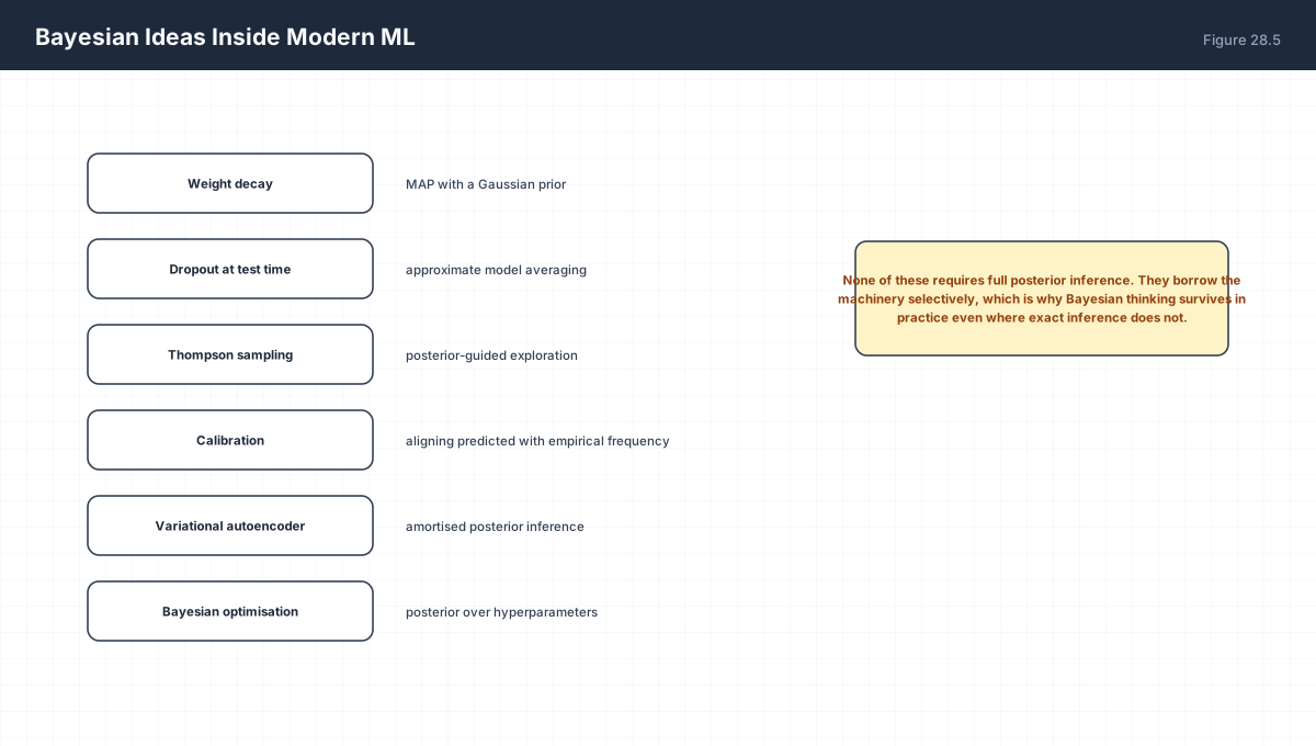
| Relevance | Dismissed as “not deep learning”. | Six places the machinery appears in modern practice. |
Core learning objectives. After this chapter you should be able to:
- Write Bayes’ theorem and name posterior, likelihood, prior, and evidence.
- Compute a posterior from base rate and test accuracy.
- Explain why a 99%-accurate test can yield a 17% posterior.
- Show that sequential updating is order-independent.
- Contrast the Bayesian and frequentist interpretations of an interval.
- Identify Bayesian machinery inside regularisation, dropout, and calibration.
2. The Formula
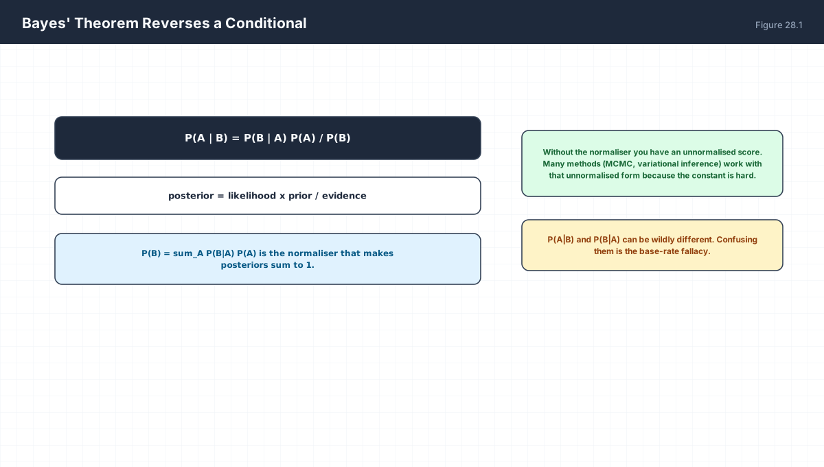
P(A | B) = P(B | A) P(A) / P(B)

posterior  = likelihood x prior / evidence

evidence   P(B) = sum_A P(B | A) P(A)
           the normaliser that makes posteriors sum to 1
import numpy as np

def posterior(prior, sensitivity, false_positive):
    """P(disease | positive test) from a base rate."""
    p_pos = sensitivity * prior + false_positive * (1 - prior)
    return sensitivity * prior / p_pos

for base in (0.001, 0.01, 0.10, 0.50):
    p = posterior(base, 0.99, 0.05)
    print(f"base rate {base:6.1%}  ->  posterior {p:7.2%}")
The function is short enough to internalise. Almost every surprise in medical screening, fraud detection, and anomaly alerting comes from the fact that prior is small while the false-positive rate is not.
3. Counting the Base Rate
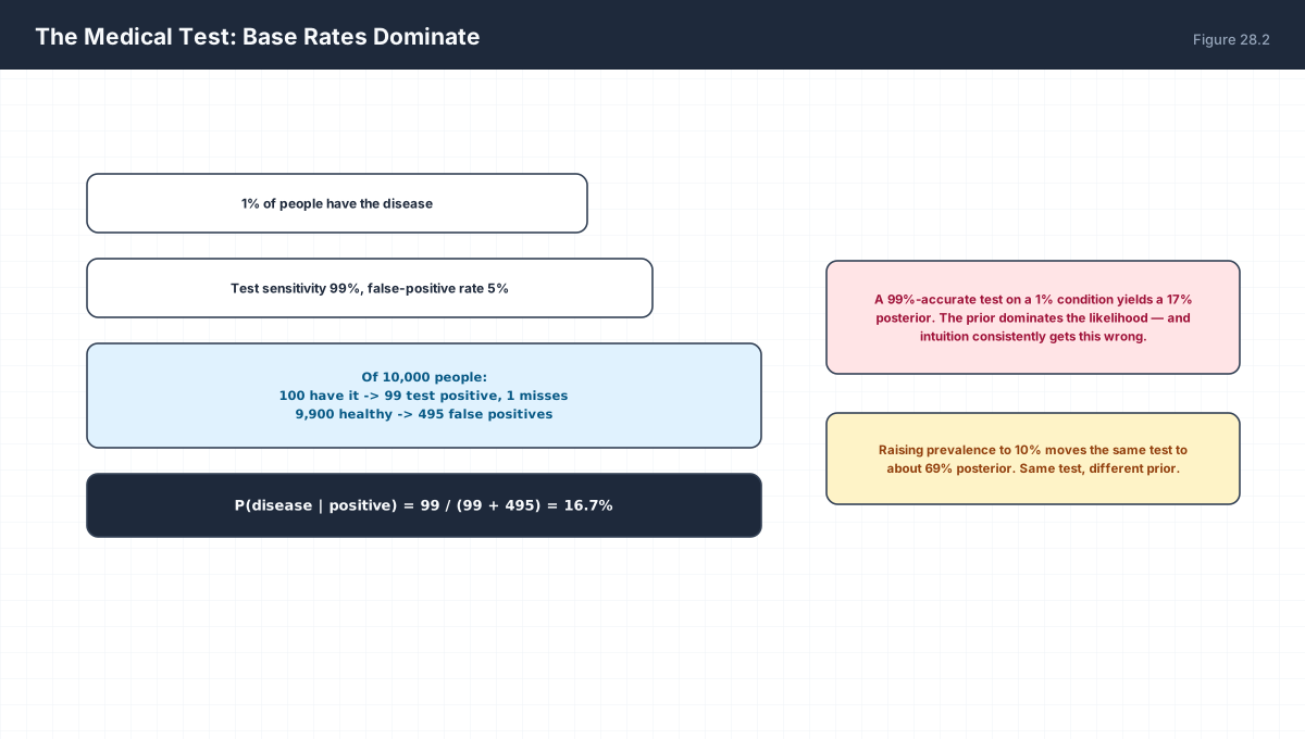
10,000 people, 1% prevalence:
    100 diseased  ->  99 test positive,  1 false negative
  9,900 healthy    ->  495 false positives

P(disease | positive) = 99 / (99 + 495) = 0.167
import numpy as np

n = 10_000
prevalence, sens, fpr = 0.01, 0.99, 0.05

diseased = int(n * prevalence)
healthy = n - diseased

true_pos = diseased * sens
false_pos = healthy * fpr

print(f"true positives : {true_pos:8.1f}")
print(f"false positives: {false_pos:8.1f}")
print(f"posterior      : {true_pos / (true_pos + false_pos):8.4f}")

# the counting answer matches the formula
formula = sens * prevalence / (sens * prevalence + fpr * (1 - prevalence))
assert np.isclose(true_pos / (true_pos + false_pos), formula)
print("counting and formula agree")
This is the whole argument for reporting sensitivity and specificity alongside prevalence. A test’s accuracy is not a property of the test alone — it is a property of the test applied to a population.
4. Sequential Updating
import numpy as np

def beta_posterior(alpha, beta, successes, failures):
    return alpha + successes, beta + failures

prior = (2.0, 2.0)                     # Beta(2,2) prior, mean 0.5

# update in one batch
a1, b1 = beta_posterior(*prior, 6, 2)

# update sequentially, one observation at a time
a2, b2 = prior
for outcome in [1, 1, 1, 1, 1, 1, 0, 0]:
    if outcome:
        a2 += 1
    else:
        b2 += 1

print("batch      :", (a1, b1), " mean", round(a1 / (a1 + b1), 6))
print("sequential :", (a2, b2), " mean", round(a2 / (a2 + b2), 6))
assert (a1, b1) == (a2, b2)
print("order and batching make no difference")
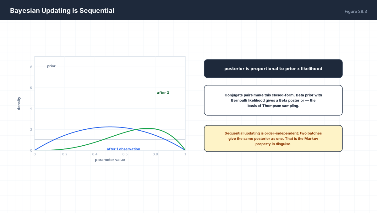
This is the conjugacy property: a Beta prior with a Bernoulli likelihood produces a Beta posterior, and the update is just counting. Thompson sampling exploits it directly — sample a parameter from the posterior, act greedily on that sample, and the exploration rate adjusts automatically as evidence accumulates.
5. Bayesian Versus Frequentist
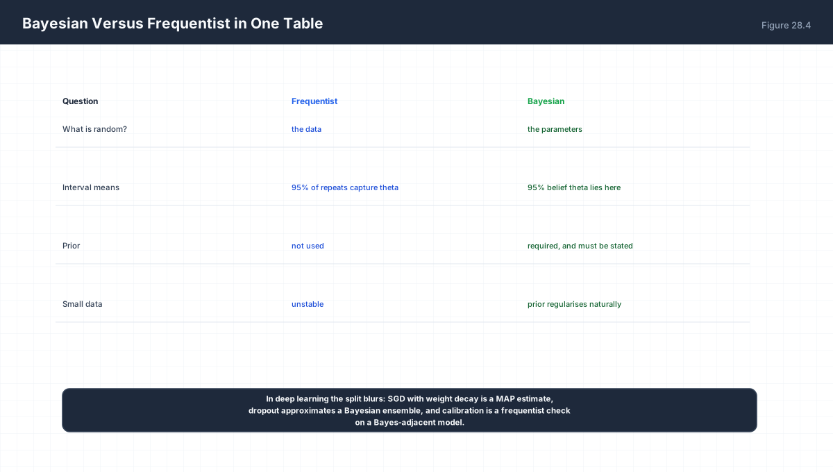
| Question | Frequentist | Bayesian |
|---|---|---|
| What is random? | The data | The parameters |
| 95% interval means | 95% of repeated samples capture θ | 95% belief that θ lies in this range |
| Prior | Not used | Required, and must be stated |
In deep learning the distinction blurs productively. Training with weight decay is maximum a posteriori estimation under a Gaussian prior — a Bayesian procedure. Evaluating calibration compares predicted probabilities against empirical frequencies — a frequentist check. Neither label is doing much work in practice; the useful question is which assumption you are willing to state.
6. Bayesian Ideas in Modern ML
import numpy as np

# Thompson sampling for a two-armed bandit
rng = np.random.default_rng(0)
true_rates = np.array([0.25, 0.40])

alpha = np.ones(2)
beta = np.ones(2)
pulls = np.zeros(2)

for _ in range(2000):
    sample = rng.beta(alpha, beta)          # draw from each posterior
    arm = int(np.argmax(sample))            # act greedily on the sample
    reward = rng.random() < true_rates[arm]
    alpha[arm] += reward
    beta[arm] += 1 - reward
    pulls[arm] += 1

print("pulls per arm:", pulls.astype(int))
print("posterior means:", np.round(alpha / (alpha + beta), 4))
print("true rates     :", true_rates)
After 2,000 pulls the algorithm has concentrated on the better arm while still allocating some pulls to the worse one — exploration proportional to remaining uncertainty, with no explicit epsilon to tune.
7. Worked Examples
7.1 Spam filter
P(spam) = 0.3
P("free" | spam)   = 0.8
P("free" | ham)    = 0.1

P("free") = 0.8(0.3) + 0.1(0.7) = 0.24 + 0.07 = 0.31
P(spam | "free") = 0.24 / 0.31 = 0.774
7.2 Two tests
Posterior after one positive: 0.167
Use that as the new prior and test again:
P = 0.99(0.167) / [0.99(0.167) + 0.05(0.833)] = 0.165/0.207 = 0.798
Two independent positives move belief from 1% to 80%.
7.3 When the prior dominates
With base rate 0.1%, even a perfect test (sens 1.0, fpr 0.0)
gives posterior 1.0 — but with fpr 1% it gives
0.001/(0.001 + 0.0099) = 9.2%.
7.4 Beta-Bernoulli update
Beta(1,1) prior (uniform)
7 successes, 3 failures  ->  Beta(8, 4)
Posterior mean = 8/12 = 0.667
MLE would say 0.700; the prior pulls it toward 0.5.
7.5 Naive Bayes
P(class | features) proportional to
  P(class) x product_i P(feature_i | class)
The independence assumption is wrong but the ranking often survives.
8. Verify It in Python
import numpy as np

# --- 1. posterior from a base rate -------------------------------
def post(prior, sens, fpr):
    return sens * prior / (sens * prior + fpr * (1 - prior))

p = post(0.01, 0.99, 0.05)
assert abs(p - 0.1667) < 0.001
print("posterior for 1% base rate:", round(p, 4))

# --- 2. counting matches the formula -----------------------------
tp, fp = 0.99 * 100, 0.05 * 9900
assert abs(tp / (tp + fp) - p) < 1e-9
print("counting and formula agree")

# --- 3. posterior grows with base rate ---------------------------
ps = [post(b, 0.99, 0.05) for b in (0.001, 0.01, 0.1, 0.5)]
assert all(x < y for x, y in zip(ps, ps[1:]))
print("posteriors increasing:", [round(x, 3) for x in ps])

# --- 4. a second independent positive compounds ---------------
p2 = post(p, 0.99, 0.05)
assert p2 > 0.7
print("after a second positive:", round(p2, 4))

# --- 5. sequential equals batch ---------------------------------
a, b = 2.0, 2.0
for outcome in (1, 1, 1, 1, 1, 1, 0, 0):
    a, b = a + outcome, b + (1 - outcome)
assert (a, b) == (8.0, 4.0)
print("Beta(2,2) + 6 successes, 2 failures ->", (a, b))

# --- 6. posterior sums to one over hypotheses -------------------
hyps = np.array([0.2, 0.5, 0.8])
prior = np.array([0.25, 0.5, 0.25])
lik = np.array([0.1, 0.6, 0.9])
raw = prior * lik
post_h = raw / raw.sum()
assert np.isclose(post_h.sum(), 1.0)
print("normalised posteriors:", np.round(post_h, 4))

# --- 7. Thompson sampling concentrates on the better arm -------
rng = np.random.default_rng(1)
rates = np.array([0.2, 0.45])
al, be = np.ones(2), np.ones(2)
pulls = np.zeros(2)
for _ in range(1500):
    arm = int(np.argmax(rng.beta(al, be)))
    r = rng.random() < rates[arm]
    al[arm] += r; be[arm] += 1 - r; pulls[arm] += 1
assert pulls[1] > pulls[0]
print("pulls:", pulls.astype(int), " -> better arm favoured")
print("all assertions passed")
9. Practice Questions
- Write Bayes' theorem and name all four terms.
- Compute the posterior for a 99% sensitive, 5% FPR test at 1% prevalence.
- Explain in one sentence why a high-accuracy test can be misleading.
- Recompute with 10% prevalence and compare.
- Show that a Beta prior plus Bernoulli data stays Beta.
- Why is sequential updating order-independent?
- State one difference between a confidence and a credible interval.
- Express weight decay as a MAP estimate.
- Explain the naive Bayes independence assumption and why it still works.
- How does Thompson sampling balance exploration and exploitation?
10. Official References & Further Reading
Continue the Course
- Course Index: AI Mathematics Masterclass — All 48 Chapters
- Previous Chapter: Chapter 27: Expectation, Variance & Covariance
- Next Chapter: Chapter 29: Maximum Likelihood & Maximum A Posteriori Estimation
- Related Series: PyTorch Engineering Masterclass — All 16 Modules