
AI Reading
Quick summary of this article
AI Mathematics Masterclass — Chapter 23 of 48
Every optimiser in deep learning is a modification of one rule: step against the gradient. The modifications exist because that rule has three weaknesses — it uses one step size for every coordinate, it ignores the history of previous steps, and it treats all directions as equally trustworthy. This chapter builds momentum, RMSProp, and Adam in sequence, showing exactly which weakness each one addresses and what it costs.
1. Technical Audit & Core Learning Objectives
| Component | Common Tutorial Deficiency | Engineering Standard Applied Here |
|---|---|---|
| Plain descent | Presented as complete, with weaknesses unstated. | Its three specific failures named first, so each fix has a target. |
| Momentum | Given as a formula without the averaging interpretation. | Framed as an exponential average with effective step η/(1−β). |
| Adam | Defaults quoted, bias correction unexplained. | Bias correction derived as the fix for a zero-initialised accumulator. |
| Batch size | Treated as a hyperparameter with no analysis. | Variance scaling made explicit, with the diminishing-returns caveat. |
Core learning objectives. After this chapter you should be able to:
- Write the plain descent update and state its three weaknesses.
- Derive momentum’s effective step size along a consistent direction.
- Implement Adam including bias correction and explain why correction is needed.
- Predict how gradient variance scales with batch size.
- Explain what each optimiser state costs in memory.
- Choose an optimiser and justify the choice.
2. Plain Gradient Descent
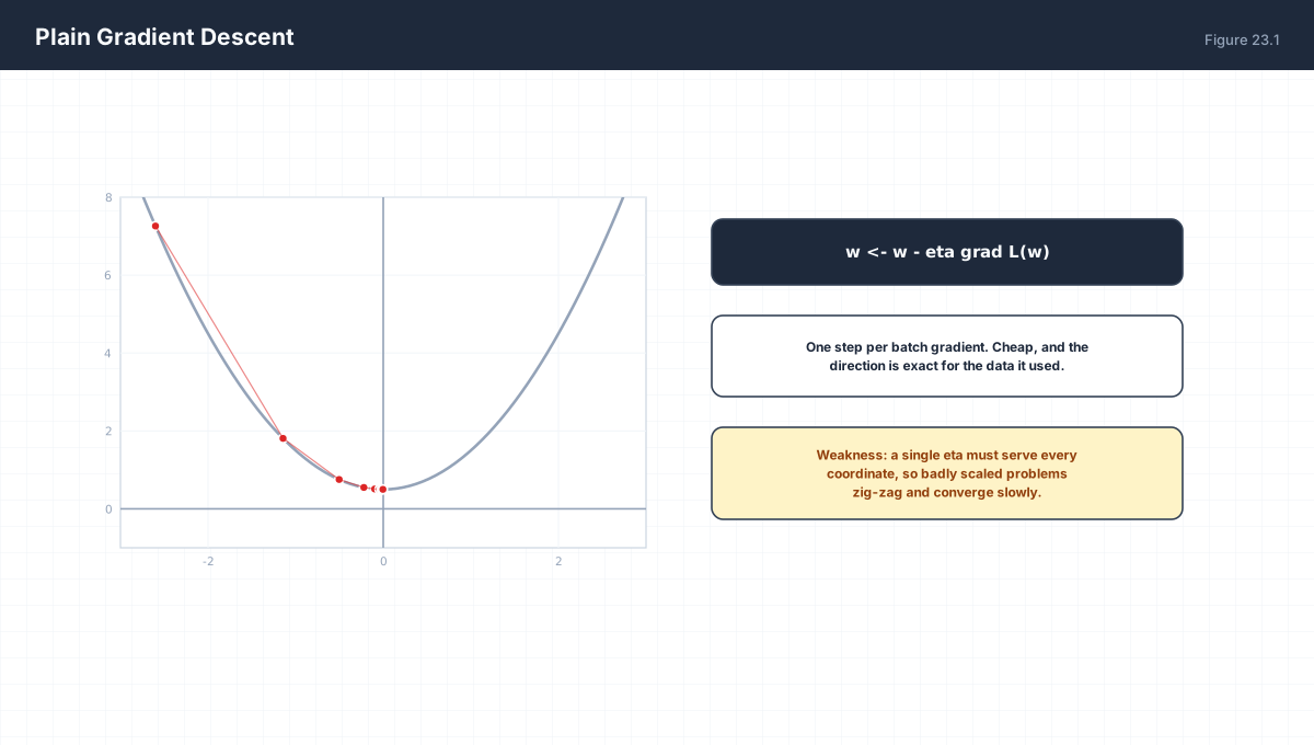
theta <- theta - eta * grad L(theta)

Three weaknesses:
  1. one global eta for every coordinate, whatever its scale
  2. no memory: each step ignores the previous ones
  3. every coordinate gets the same trust, even if its
     gradient is far noisier than its neighbour's
import numpy as np

def gd(grad, theta0, eta, steps):
    theta = np.array(theta0, dtype=float)
    for _ in range(steps):
        theta = theta - eta * grad(theta)
    return theta

# ill-conditioned quadratic: curvature 1 vs 100
A = np.array([[1.0, 0.0], [0.0, 100.0]])
grad = lambda t: A @ t

theta = gd(grad, [1.0, 1.0], eta=0.015, steps=200)
print("final:", np.round(theta, 8))
print("eta ceiling is 2/100 = 0.02; the first axis then moves at", 1 - 0.015 * 1.0, "per step")
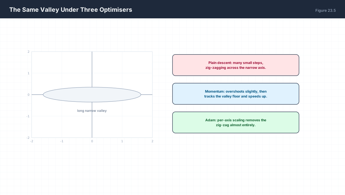
With curvature 100 on the second axis and 1 on the first, stability forces η < 0.02, but at that rate the first axis contracts by only 1.5% per step. Reaching an error of 1e-8 on that axis alone takes roughly 1,200 steps. This factor-of-100 mismatch is what momentum and adaptive methods are for.
3. Momentum
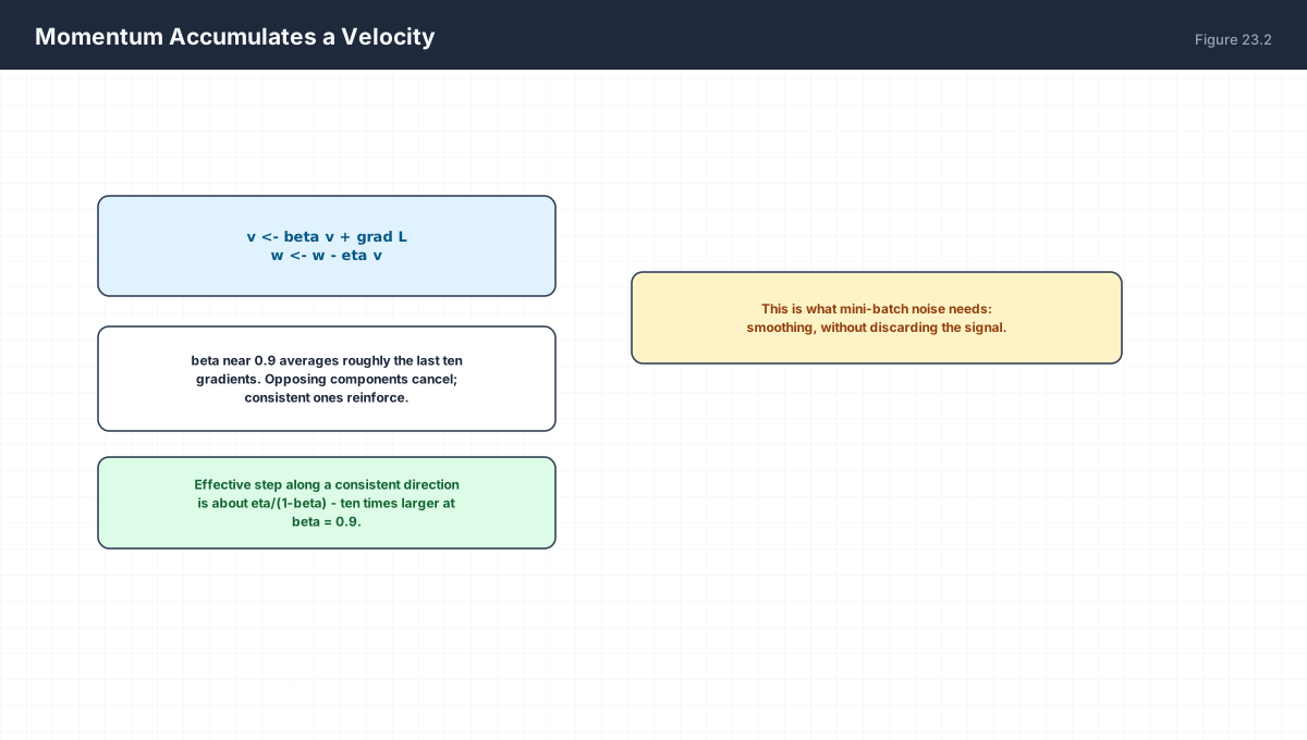
v <- beta * v + grad L
theta <- theta - eta * v

beta = 0 draws plain descent.
beta = 0.9 averages roughly the last 1/(1-beta) = 10 gradients.

Along a consistent direction the velocity reaches grad/(1-beta),
so the effective step is eta/(1-beta) — ten times larger at 0.9.
Across a valley the oscillations cancel, because consecutive
gradients point in opposite directions.
import numpy as np

def momentum(grad, theta0, eta, beta, steps):
    theta = np.array(theta0, dtype=float)
    v = np.zeros_like(theta)
    for _ in range(steps):
        v = beta * v + grad(theta)
        theta = theta - eta * v
    return theta

A = np.array([[1.0, 0.0], [0.0, 100.0]])
grad = lambda t: A @ t

# same eta as before, but momentum reaches the basin much faster
for beta in (0.0, 0.9, 0.99):
    t = momentum(grad, [1.0, 1.0], eta=0.015, beta=beta, steps=200)
    print(f"beta={beta:4.2f}  final norm={np.linalg.norm(t):.3e}")
Momentum does not remove the stability constraint — it lowers it slightly, requiring η < 2(1+β)/λmax. What it does is convert the slow direction into a faster one by accumulating consistent steps, while cancelling the oscillatory ones.
4. Adam
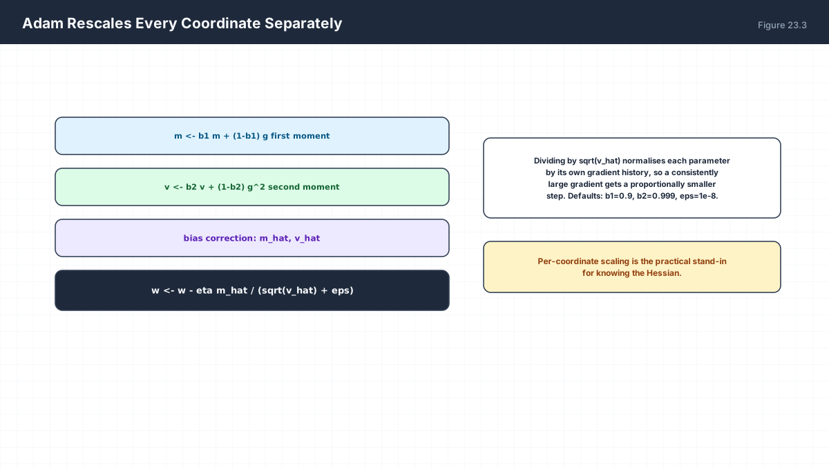
m <- b1*m + (1-b1)*g           first moment  (momentum)
v <- b2*v + (1-b2)*g^2         second moment (magnitude)
m_hat = m / (1 - b1^t)         bias correction
v_hat = v / (1 - b2^t)
theta <- theta - eta * m_hat / (sqrt(v_hat) + eps)

Defaults: b1 = 0.9, b2 = 0.999, eps = 1e-8
Bias correction exists for one reason: v starts at zero and is updated by (1−β₂)g², so after one step it equals 0.001·g², not g². Dividing by 1−β₂ᵗ rescales it back. Without correction, the first few steps would be enormous — η/sqrt(0.001) ≈ 31η instead of η.
import numpy as np

def adam(grad, theta0, eta=0.01, b1=0.9, b2=0.999, eps=1e-8, steps=500):
    theta = np.array(theta0, dtype=float)
    m = np.zeros_like(theta); v = np.zeros_like(theta)
    for t in range(1, steps + 1):
        g = grad(theta)
        m = b1 * m + (1 - b1) * g
        v = b2 * v + (1 - b2) * g ** 2
        m_hat = m / (1 - b1 ** t)
        v_hat = v / (1 - b2 ** t)
        theta = theta - eta * m_hat / (np.sqrt(v_hat) + eps)
    return theta

A = np.array([[1.0, 0.0], [0.0, 100.0]])
result = adam(lambda t: A @ t, [1.0, 1.0])
print("adam final:", np.round(result, 10), " norm:", f"{np.linalg.norm(result):.2e}")

# the same eta works on a much worse-conditioned problem
B = np.diag([0.01, 1000.0])
result2 = adam(lambda t: B @ t, [1.0, 1.0], eta=0.01, steps=2000)
print("kappa=100000 case:", np.round(result2, 8))
5. Batch Size and Gradient Noise
import numpy as np

rng = np.random.default_rng(0)
true_grad = np.array([1.0, -2.0, 0.5])
noise = 1.0

print(f"{'batch':>6} {'std of mean grad':>18}")
for k in (1, 4, 16, 64, 256, 1024):
    samples = true_grad + rng.normal(0, noise, size=(4000, k, 3))
    means = samples.mean(axis=1)
    print(f"{k:6d} {means.std(axis=0).mean():18.4f}")
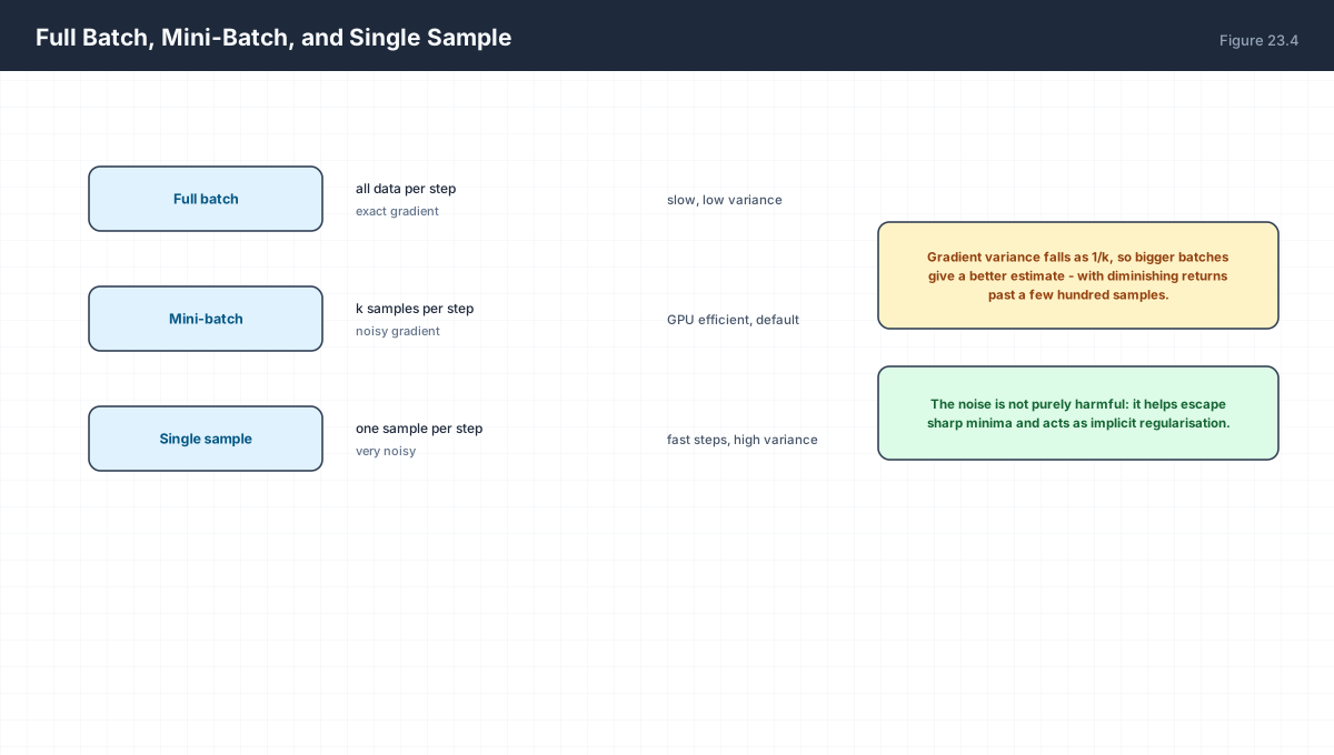
print("\nvariance falls as 1/k, so std falls as 1/sqrt(k)")
Standard deviation halves when batch size quadruples, which is the diminishing return: going from 256 to 1024 costs 4× the compute for 2× the gradient precision. Beyond a few hundred samples, the wall-clock cost dominates the benefit, which is why mini-batches in the tens-to-hundreds range are standard.
6. Optimiser State and Memory
| Optimiser | Extra State | × Model Size |
|---|---|---|
| SGD | none | 0 |
| Momentum | velocity v |
1× |
| Adam | m and v |
2× |
| AdamW | m and v, decoupled decay |
2× |
params = 1_000_000_000
for name, mult in (("SGD", 0), ("Momentum", 1), ("Adam", 2)):
    weights = params * 4 / 1e9          # float32
    opt = params * 4 * mult / 1e9
    print(f"{name:10s} weights {weights:5.1f} GB  optimiser {opt:5.1f} GB  total {weights+opt:5.1f} GB")
A billion-parameter model in float32 needs 4 GB for weights and 8 GB more for Adam's state — before activations. This is why mixed precision and 8-bit optimisers exist: the optimiser state, not the weights, is often the dominant memory cost.
7. Worked Examples
7.1 Effective momentum step
beta = 0.9, eta = 0.01, constant gradient g
Steady-state velocity = g/(1-0.9) = 10g
Effective step = 0.01 * 10g = 0.1g    ten times the plain step
7.2 Bias correction at t = 1
v_1 = 0.001 * g^2
1 - b2^1 = 0.001
v_hat = 0.001 g^2 / 0.001 = g^2       exactly right
7.3 Why Adam handles scale
Coordinate A: gradient 100.   m/sqrt(v) ~ 1
Coordinate B: gradient 0.01.  m/sqrt(v) ~ 1
Both get a step of about eta. The ratio of 10,000 disappears.
7.4 AdamW versus Adam
Adam:  theta <- theta - eta*(m_hat/(sqrt(v_hat)+eps) + wd*theta)
AdamW: theta <- theta - eta*m_hat/(sqrt(v_hat)+eps) - eta*wd*theta
In Adam the decay is scaled by the adaptive denominator, so it is
not a uniform pull toward zero. Decoupling fixes that.
7.5 Batch size and steps
Doubling the batch halves the number of steps per epoch but roughly
halves the gradient variance. Practitioners often scale eta with
sqrt(batch) or linearly, depending on the regime.
8. Verify It in Python
import numpy as np

A = np.array([[1.0, 0.0], [0.0, 100.0]])

def gd(theta0, eta, steps=2000):
    t = np.array(theta0, float)
    for _ in range(steps):
        t = t - eta * (A @ t)
    return t

def mom(theta0, eta, beta, steps=500):
    t = np.array(theta0, float); v = np.zeros_like(t)
    for _ in range(steps):
        v = beta * v + A @ t
        t = t - eta * v
    return t

def adam(theta0, eta=0.01, b1=0.9, b2=0.999, eps=1e-8, steps=2000):
    t = np.array(theta0, float)
    m = np.zeros_like(t); v = np.zeros_like(t)
    for k in range(1, steps + 1):
        g = A @ t
        m = b1 * m + (1 - b1) * g
        v = b2 * v + (1 - b2) * g ** 2
        t = t - eta * (m / (1 - b1 ** k)) / (np.sqrt(v / (1 - b2 ** k)) + eps)
    return t

# --- 1. plain descent is limited by the steep axis ---------------
assert np.linalg.norm(gd([1., 1.], 0.015)) < 1e-8
with np.errstate(over="ignore", invalid="ignore"):
    bad = gd([1., 1.], 0.03)               # eta*lambda_max = 3 > 2 -> diverges
diverged = (not np.all(np.isfinite(bad))) or np.linalg.norm(bad) > 1.0
assert diverged
print("plain descent: stable at 0.015, diverges at 0.03")

# --- 2. momentum accelerates the flat direction ------------------
n_plain = np.linalg.norm(gd([1., 1.], 0.015, steps=60))
n_mom = np.linalg.norm(mom([1., 1.], 0.015, 0.9, steps=60))
assert n_mom < n_plain
print(f"after 60 steps: plain={n_plain:.3e}  momentum={n_mom:.3e}")

# --- 3. Adam reaches machine precision --------------------------
adm = adam([1., 1.])
assert np.linalg.norm(adm) < 1e-6
print("adam final norm:", f"{np.linalg.norm(adm):.2e}")

# --- 4. Adam handles extreme conditioning -----------------------
B = np.diag([0.01, 1000.0])
def adam_B(theta0, eta=0.01, steps=3000):
    t = np.array(theta0, float)
    m = np.zeros_like(t); v = np.zeros_like(t)
    b1, b2, eps = 0.9, 0.999, 1e-8
    for k in range(1, steps + 1):
        g = B @ t
        m = b1 * m + (1 - b1) * g
        v = b2 * v + (1 - b2) * g ** 2
        t = t - eta * (m / (1 - b1 ** k)) / (np.sqrt(v / (1 - b2 ** k)) + eps)
    return t
assert np.linalg.norm(adam_B([1., 1.])) < 1e-4
print("adam on kappa=1e5:", np.round(adam_B([1., 1.]), 8))

# --- 5. bias correction is exact at t = 1 -----------------------
g = 3.0
b2 = 0.999
v = (1 - b2) * g ** 2
assert np.isclose(v / (1 - b2), g ** 2)
print("bias correction recovers g^2 exactly at t=1")

# --- 6. gradient noise falls as 1/sqrt(k) -----------------------
rng = np.random.default_rng(0)
stds = {}
for k in (1, 16, 256):
    means = (1.0 + rng.normal(0, 1.0, size=(4000, k))).mean(axis=1)
    stds[k] = means.std()
assert stds[256] < stds[16] < stds[1]
assert np.isclose(stds[256] / stds[1], 1 / np.sqrt(256), rtol=0.15)
print("noise scaling:", {k: round(v, 4) for k, v in stds.items()})

# --- 7. optimizer memory arithmetic ----------------------------
params = 1_000_000_000
weights_gb = params * 4 / 1e9
adam_extra_gb = params * 8 / 1e9
assert np.isclose(weights_gb, 4.0) and np.isclose(adam_extra_gb, 8.0)
print(f"1B params: {weights_gb:.0f} GB weights + {adam_extra_gb:.0f} GB Adam state")
print("all assertions passed")
9. Practice Questions
- State the three weaknesses of plain gradient descent.
- With
β = 0.9, how many past gradients does momentum effectively average? - Show that steady-state momentum step size is
η/(1−β)times the gradient. - Why is bias correction necessary in Adam, and when does it stop mattering?
- Explain how Adam makes a 10,000× scale difference between coordinates irrelevant.
- Compute Adam's memory overhead for a 7-billion-parameter model in float32.
- Why does gradient standard deviation halve when batch size quadruples?
- What is the practical limit on increasing batch size?
- Contrast Adam and AdamW weight decay.
- Given
λmax = 50, state the largest stable plain-descent learning rate.
10. Official References & Further Reading
Continue the Course
- Course Index: AI Mathematics Masterclass — All 48 Chapters
- Previous Chapter: Chapter 22: Jacobians, Hessians & Second-Order Geometry
- Next Chapter: Chapter 24: Convexity, Constraints & Lagrange Multipliers
- Related Series: PyTorch Engineering Masterclass — All 16 Modules