
AI Reading
Quick summary of this article
AI Mathematics Masterclass — Chapter 13 of 48
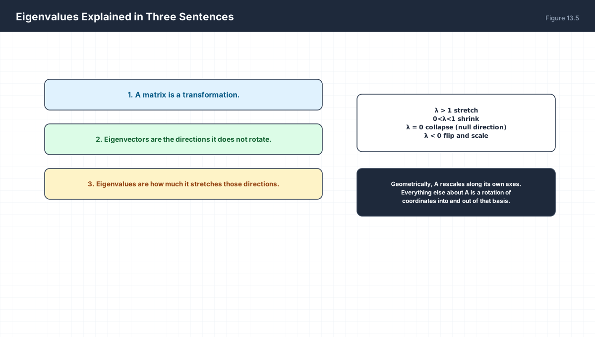
An eigenvector is a direction a matrix does not rotate. An eigenvalue is how much it stretches along that direction. That is the entire concept, and it explains why covariance matrices have real eigenvalues, why power iteration converges, why spectral normalization stabilises GANs, and why “the largest eigenvalue” is the most consequential number in a training run. This chapter derives the characteristic polynomial, works the 2×2 case completely, and reads the spectrum as a diagnostic.
1. Technical Audit & Core Learning Objectives
| Component | Common Tutorial Deficiency | Engineering Standard Applied Here |
|---|---|---|
| Definition | Av = λv stated algebraically, never pictured. |
Drawn: unchanged direction, changed length. |
| Computation | 2×2 example only; never extended to why you’d use a library. | Characteristic polynomial derived, then eig/eigh used appropriately. |
| Properties | Symmetric ⇒ real eigenvalues asserted without use. | Tied to covariance matrices and PCA’s well-definedness. |
| Diagnostics | Spectral radius never mentioned. | Linked to gradient explosion and spectral normalisation. |
Core learning objectives. After this chapter you should be able to:
- Verify by direct multiplication whether a vector is an eigenvector.
- Derive the characteristic polynomial and solve it for a 2×2 matrix.
- Use
sum(λ) = traceandprod(λ) = detas consistency checks. - Diagonalize a matrix as
PΛP⁻¹and explain what that buys you. - State the spectral properties of symmetric, orthogonal, and positive-definite matrices.
- Explain spectral radius and why it governs stability.
2. The Definition, Geometrically
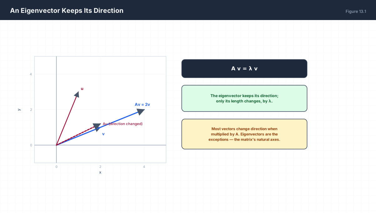
A v = λ v          v ≠ 0,  λ is a scalar

Reading: multiplying by A has the same effect as scaling by λ,
for this particular direction only.

λ > 1     stretch
0 < λ < 1 shrink
λ = 0     collapse to zero  →  v is in the null space
λ < 0     flip direction and scale
λ = 1     unchanged  →  v is a fixed point of A
import numpy as np

A = np.array([[2.0, 1.0], [1.0, 2.0]])
v = np.array([1.0, 1.0])

print("A @ v      :", A @ v)                 # [3. 3.]
print("lambda * v :", 3.0 * v)               # [3. 3.]
assert np.allclose(A @ v, 3.0 * v)
print("(1,1) is an eigenvector with lambda = 3")

u = np.array([1.0, 3.0])
Au = A @ u
parallel = np.isclose(np.linalg.det(np.column_stack([Au, u])), 0.0)
print("A @ u:", Au, " parallel to u?", parallel)     # False, so u is NOT an eigenvector
3. Finding Eigenvalues
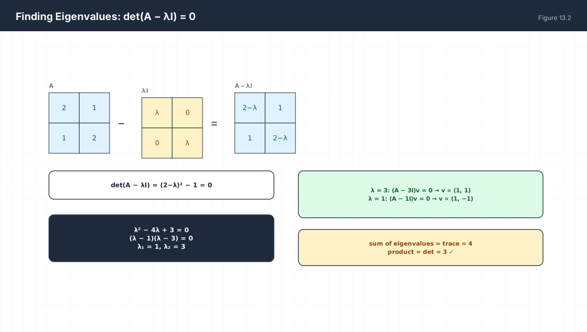
The equation Av = λv rearranges to (A − λI)v = 0. A non-zero v exists only if that matrix is singular, which is exactly the determinant condition.
det(A − λI) = 0

For A = [[2,1],[1,2]]:
  A − λI = [[2−λ, 1], [1, 2−λ]]
  det = (2−λ)² − 1 = λ² − 4λ + 3
  roots: λ = 1, λ = 3

Check:  sum = 4 = trace(A)      product = 3 = det(A)
import numpy as np

A = np.array([[2.0, 1.0], [1.0, 2.0]])
vals, vecs = np.linalg.eig(A)
print("eigenvalues :", np.round(vals.real, 6))     # [3. 1.]
print("eigenvectors:\n", np.round(vecs.real, 4))

print("trace check  :", round(float(vals.real.sum()), 6), "==", np.trace(A))
print("det check    :", round(float(np.prod(vals.real)), 6), "==", round(np.linalg.det(A), 6))

# symmetric matrices: use eigh for real, sorted, orthonormal output
vals_s, vecs_s = np.linalg.eigh(A)
print("eigh sorted  :", np.round(vals_s, 6))
assert np.allclose(vecs_s.T @ vecs_s, np.eye(2))
Use eigh rather than eig whenever the matrix is symmetric. It guarantees real eigenvalues, returns them sorted, and produces orthonormal eigenvectors — all facts that eig cannot guarantee for a general matrix.
4. Which Matrices Have Predictable Spectra
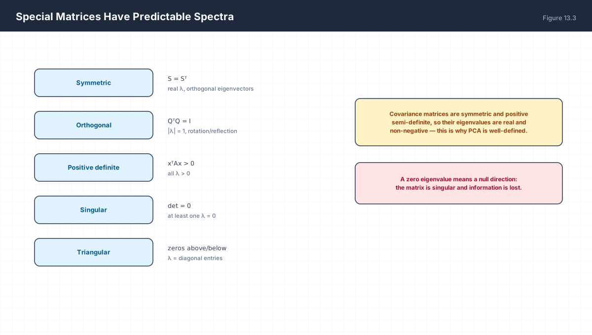
| Type | Guarantee | Consequence |
|---|---|---|
| Symmetric | Real λ, orthogonal eigenvectors | Always diagonalizable; PCA is well-defined |
| Positive definite | All λ > 0 | Strictly convex loss; unique minimum |
| Orthogonal | |λ| = 1 |
Preserves norms; no amplification |
| Singular | At least one λ = 0 | Non-trivial null space; non-invertible |
| Triangular | λ = diagonal entries | Read off directly, no computation |
import numpy as np

S = np.array([[4.0, 2.0], [2.0, 3.0]])
print("symmetric, real λ:", np.round(np.linalg.eigvalsh(S), 4))

O = np.array([[0.0, -1.0], [1.0, 0.0]])
print("orthogonal, |λ|=1:", np.round(np.abs(np.linalg.eigvals(O)), 6))

D = np.array([[3.0, 0.0], [0.0, 0.5]])
print("positive definite:", np.all(np.linalg.eigvalsh(D) > 0))

Z = np.array([[1.0, 2.0], [2.0, 4.0]])
print("singular, min |λ|:", round(np.abs(np.linalg.eigvals(Z)).min(), 10))
5. Diagonalization
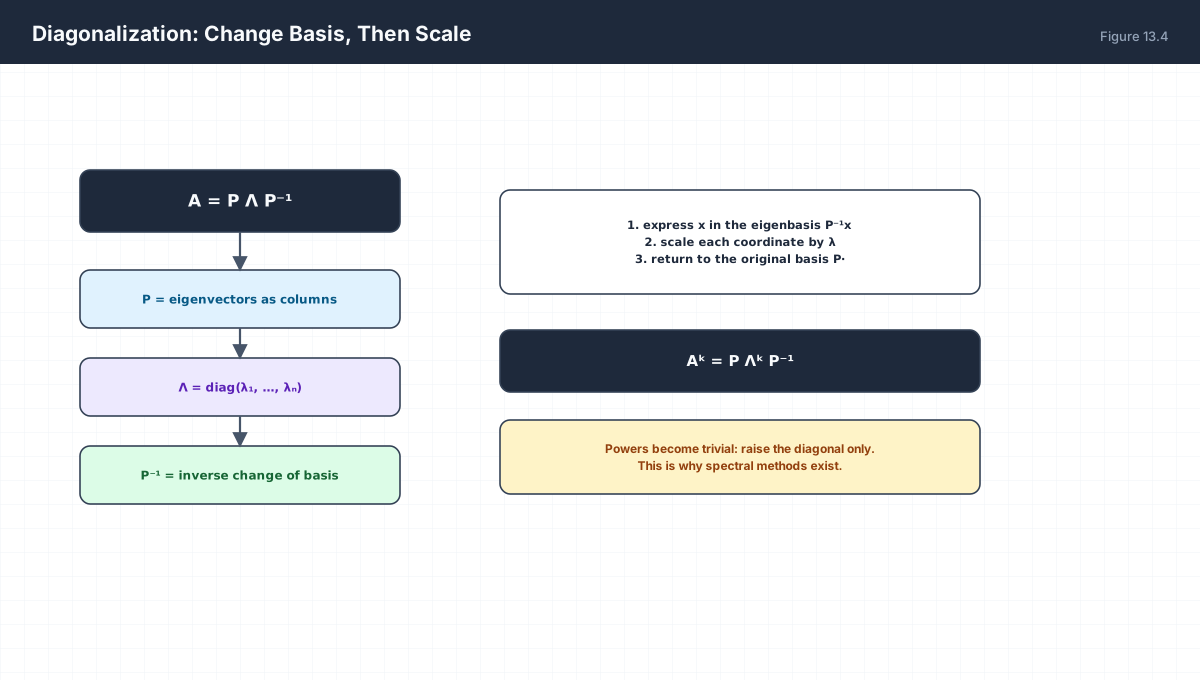
A = P Λ P⁻¹        P = [v₁ v₂ … vₙ] as columns,  Λ = diag(λ)

Meaning:
  P⁻¹ x     express x in the eigenbasis
  Λ (…)     scale each coordinate independently
  P (…)     return to the original basis

Consequence:
  Aᵏ = P Λᵏ P⁻¹        so Aᵏ is governed entirely by λᵏ
import numpy as np

A = np.array([[2.0, 1.0], [1.0, 2.0]])
vals, P = np.linalg.eigh(A)
Lam = np.diag(vals)

rebuilt = P @ Lam @ P.T                 # symmetric: P⁻¹ == Pᵀ
print("A reproduced:", np.allclose(rebuilt, A))

# powers are cheap in the eigenbasis
print("A^10 == P Λ^10 Pᵀ:", np.allclose(np.linalg.matrix_power(A, 10), P @ np.diag(vals**10) @ P.T))

# spectral radius governs whether A^k blows up or decays
print("spectral radius:", round(np.abs(vals).max(), 4))
Symmetric matrices are especially convenient because P⁻¹ = Pᵀ, so the decomposition costs nothing to invert. For non-symmetric matrices P may be badly conditioned, and the reconstruction is numerically fragile even when exact in theory.
6. Spectral Radius and Stability
The spectral radius ρ(A) = max|λᵢ| determines what happens under repeated application:
| Spectral Radius | Behaviour of Aᵏx | In Training |
|---|---|---|
ρ < 1 |
Decays to zero | Vanishing signal across layers |
ρ = 1 |
Bounded, neither grows nor decays | The target for stable deep networks |
ρ > 1 |
Grows exponentially | Exploding gradients |
import numpy as np

rng = np.random.default_rng(0)
for d in (16, 64):
    W = rng.normal(size=(d, d)) / np.sqrt(d)
    rho = np.abs(np.linalg.eigvals(W)).max()
    x = rng.normal(size=d)
    for _ in range(20):
        x = W @ x
    print(f"d={d:3d}  rho={rho:.3f}  ‖W²⁰x‖={np.linalg.norm(x):.3e}")
A weight matrix initialised with variance 1/d has ρ ≈ 1, which keeps activations bounded through depth. That is the principle behind the He and Xavier initialisation schemes — they are spectral radius arguments in disguise. Spectral normalization in GANs takes the same idea and enforces ρ = 1 explicitly at every step.
7. Worked Examples
7.1 Verify an eigenpair
A = [[4,1],[2,3]], v = (1,−1)
A v = (4−1, 2−3) = (3, −1) = 3·(1,−1)   ✓  λ = 3
7.2 Full 2×2 solve
A = [[4,1],[2,3]]
det(A − λI) = (4−λ)(3−λ) − 2 = λ² − 7λ + 10
roots: λ = 5, λ = 2
trace 4+3 = 7 = 5+2 ✓     det 12−2 = 10 = 5·2 ✓
7.3 Triangular matrix
U = [[3,7,1],[0,2,5],[0,0,−1]]
λ = 3, 2, −1     read straight off the diagonal
7.4 Eigenvalues of a projection
A projection onto a line: P² = P.
Then λ² = λ  →  λ ∈ {0, 1}.
1 means "kept", 0 means "projected away" — exactly right.
7.5 Power iteration converges to the dominant eigenvector
Repeat x ← Ax / ‖Ax‖
The component along the largest-|λ| direction grows fastest,
so x converges to that eigenvector. Ratio of convergence
is |λ₂/λ₁|.
8. Verify It in Python
import numpy as np

# --- 1. eigenpair by direct multiplication ------------------------
A = np.array([[2., 1.], [1., 2.]])
v = np.array([1., 1.])
assert np.allclose(A @ v, 3.0 * v)
print("Av == 3v verified")

# --- 2. characteristic polynomial roots ---------------------------
vals = np.linalg.eigvalsh(A)
assert np.allclose(sorted(vals), [1.0, 3.0])
assert np.isclose(vals.sum(), np.trace(A))
assert np.isclose(np.prod(vals), np.linalg.det(A))
print("eigenvalues:", np.round(vals, 6))

# --- 3. symmetric gives orthonormal eigenvectors ------------------
_, P = np.linalg.eigh(A)
assert np.allclose(P.T @ P, np.eye(2))
print("eigh returns orthonormal columns")

# --- 4. diagonalization reconstructs A ---------------------------
assert np.allclose(P @ np.diag(vals) @ P.T, A)
print("P L P^T == A")

# --- 5. powers follow lambda^k -----------------------------------
big = np.array([[4., 1.], [2., 3.]])
w, V = np.linalg.eig(big)
Vi = np.linalg.inv(V)
assert np.allclose(np.linalg.matrix_power(big, 6), V @ np.diag(w ** 6) @ Vi)
print("A^6 == P Λ^6 P^-1")

# --- 6. spectral radius predicts growth --------------------------
decay = np.diag([0.5, 0.9])
grow = np.diag([1.2, 0.9])
assert np.abs(np.linalg.eigvals(decay)).max() < 1
assert np.abs(np.linalg.eigvals(grow)).max() > 1
x = np.array([1., 1.])
for _ in range(300):                     # 0.9^300 ≈ 2e-14, so both components vanish
    x = decay @ x
assert np.linalg.norm(x) < 1e-10
print("rho<1 decays as predicted")

# --- 7. power iteration finds the dominant direction --------------
rng = np.random.default_rng(1)
M = np.diag([9.0, 5.0, 3.0, 1.5, 0.4])
M = M + 0.1 * (rng.normal(size=(5, 5)) + rng.normal(size=(5, 5)).T) / 2
x = rng.normal(size=5)
for _ in range(200):
    x = M @ x
    x = x / np.linalg.norm(x)
true_vec = np.linalg.eigh(M)[1][:, -1]
print("power iteration aligned:", round(abs(x @ true_vec), 6))
assert abs(x @ true_vec) > 0.999
print("all assertions passed")
9. Practice Questions
- Verify that
(1,−1)is an eigenvector of[[4,1],[2,3]]and give λ. - Solve
det(A − λI) = 0for[[3,1],[1,3]]and check against trace and det. - Read the eigenvalues of an upper-triangular matrix from its diagonal and justify why.
- Why does
λ = 0imply the matrix is singular? - Show that a projection matrix has eigenvalues only 0 and 1.
- Why does
|λ| = 1hold for every orthogonal matrix? - Express
Aᵏin terms ofPandΛand explain why this is useful. - State the spectral radius of
diag(0.9, 0.5, −0.7)and the behaviour of its powers. - Why does variance-1/d initialisation produce ρ ≈ 1?
- Explain power iteration's convergence rate in terms of λ₁ and λ₂.
10. Official References & Further Reading
Continue the Course
- Course Index: AI Mathematics Masterclass — All 48 Chapters
- Previous Chapter: Chapter 12: Orthogonality, Projections & Least Squares
- Next Chapter: Chapter 14: Singular Value Decomposition (SVD)
- Related Series: PyTorch Engineering Masterclass — All 16 Modules