
AI Reading
Quick summary of this article
AI Mathematics Masterclass — Chapter 46 of 48
An LLM is a tokeniser, an embedding table, a stack of transformer blocks, and a projection back to the vocabulary. This chapter works through the arithmetic of that pipeline: why subword tokenisation exists, how much of a model’s parameter budget the embedding consumes, how sampling temperature reshapes a distribution, and where the 6ND training-cost estimate comes from.
1. Technical Audit & Core Learning Objectives
| Component | Common Tutorial Deficiency | Engineering Standard Applied Here |
|---|---|---|
| Tokenisation | “It splits words” — no further detail. | BPE mechanics and the whitespace-token trap shown. |
| Embeddings | Called a “layer” with no cost analysis. | V×d counted and compared against the transformer body. |
| Sampling | Temperature mentioned without the effect. | Distribution reshape computed for three temperatures. |
| Scaling | 6ND quoted as gospel. | Derived from forward and backward FLOPs, limits stated. |
Core learning objectives. After this chapter you should be able to:
- Explain why subword tokenisation exists.
- Describe the BPE merge procedure.
- Compute an embedding table’s parameter cost.
- Explain weight tying.
- Predict the effect of temperature on a distribution.
- Derive the 6ND training-FLOP estimate.
2. Tokenisation
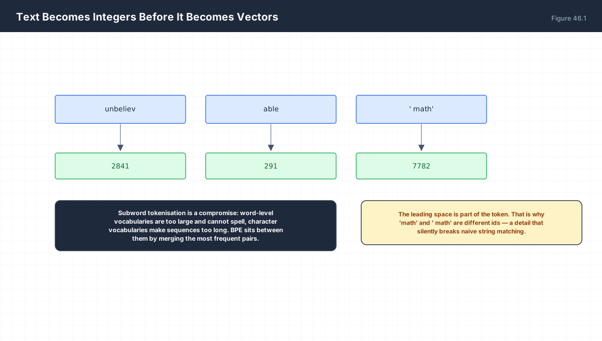
Word-level:   one id per word     -> huge vocabulary, no OOV handling
Character-level: one id per char  -> tiny vocabulary, very long sequences
Subword:      frequent words are one token, rare words split

BPE: start from characters, repeatedly merge the most frequent
adjacent pair. Stop at the target vocabulary size.

The leading space is part of the token: ' math' and 'math' are
different ids. This breaks naive substring matching.
from collections import Counter

def bpe_learn(words, vocab_size):
    """Tiny BPE: words are tuples of chars with an end marker."""
    vocab = Counter()
    for w in words:
        vocab[tuple(w) + ("",)] += 1
    merges = []
    while len(set(s for w in vocab for s in w)) < vocab_size:
        pairs = Counter()
        for w, c in vocab.items():
            for a, b in zip(w, w[1:]):
                pairs[(a, b)] += c
        if not pairs:
            break
        best = pairs.most_common(1)[0][0]
        merges.append(best)
        new_vocab = Counter()
        for w, c in vocab.items():
            out, i = [], 0
            while i < len(w):
                if i < len(w) - 1 and (w[i], w[i + 1]) == best:
                    out.append(w[i] + w[i + 1]); i += 2
                else:
                    out.append(w[i]); i += 1
            new_vocab[tuple(out)] += c
        vocab = new_vocab
    return merges, vocab

corpus = ["low", "low", "low", "lower", "newest", "newest", "widest", "lowest"]
merges, vocab = bpe_learn(corpus, 20)
print("merges learned:", merges)
print("\nsegmentation after training:")
for w in vocab:
    print("  ", " | ".join(w))
The merges are learned from frequency alone — nothing about English morphology is encoded. That is why tokenisers handle some languages and code badly: whichever substrings were frequent in the training corpus get short tokens, and everything else is split into fragments.
3. The Embedding Table
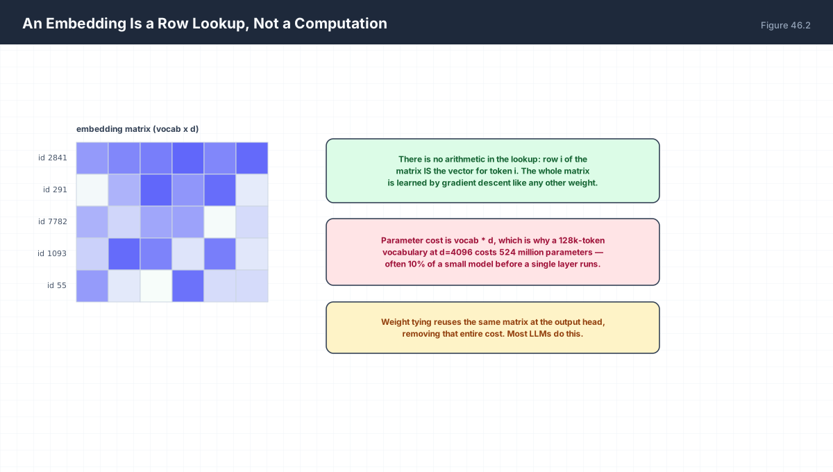
E is (vocab, d). Token id i returns row i.

Parameters = vocab * d

For vocab = 128k and d = 4096:
  128,000 * 4096 = 524,288,000  (~0.52B)

The output head is another (vocab, d) matrix unless tied.
Tying shares the two, which is why most LLMs do it.

Note the asymmetry: the embedding is a lookup (cheap, random
access) while the body is matmuls (expensive, dense).
import numpy as np

rng = np.random.default_rng(0)

def embed_cost(vocab, d):
    return vocab * d

print(f"{'vocab':>8}{'d':>7}{'embedding params':>20}")
for vocab in (32_000, 50_257, 128_000):
    for d in (4096,):
        p = embed_cost(vocab, d)
        print(f"{vocab:8,}{d:7}{p:20,}")

print()
# compare against a 7B body
d, L = 4096, 32
body = L * 12 * d * d
emb = embed_cost(128_000, d)
print(f"body params      : {body:>15,}")
print(f"embedding params : {emb:>15,}")
print(f"embedding share  : {emb/(body+emb):>14.1%}")

# a real lookup
E = rng.normal(size=(128_000, 8))
ids = np.array([2841, 291, 7782])
print("\nlookup shape:", E[ids].shape)
print("row 2841 is the vector itself:", np.allclose(E[ids][0], E[2841]))
Here the embedding is 7.5% of the total. Make the model shallower or the vocabulary larger and that share grows quickly — a 12-layer model with the same vocabulary puts it near 20%. The embedding also receives gradient on every single token, while deep layers receive it rarely. That imbalance is why tying the output matrix and using smaller vocabularies are both live design decisions.
4. Sampling
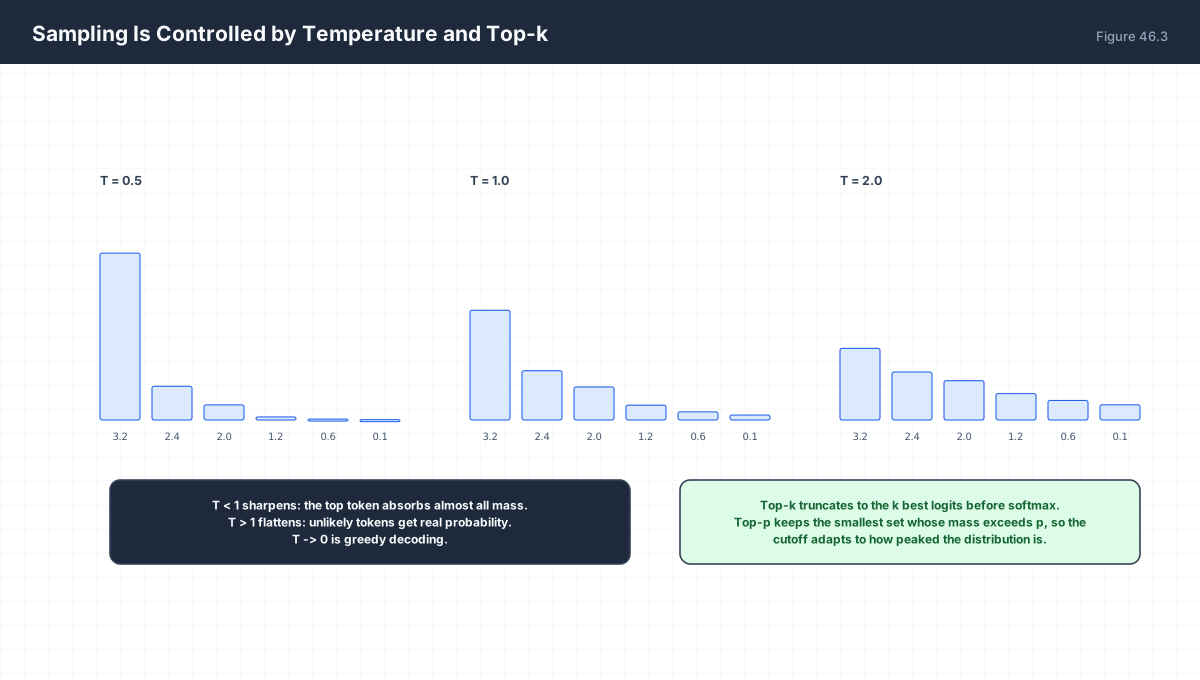
p = softmax(z / T)

T < 1  sharpens  -> closer to greedy, more repetitive
T = 1  unchanged
T > 1  flattens  -> more diverse, more incoherent

T -> 0  approaches argmax (a one-hot distribution)
T -> inf approaches uniform

top-k truncates to k logits; top-p keeps the smallest set
whose cumulative probability exceeds p.
import numpy as np

logits = np.array([3.2, 2.4, 2.0, 1.2, 0.6, 0.1])

def softmax(z):
    e = np.exp(z - z.max())
    return e / e.sum()

def entropy(p):
    p = p[p > 0]
    return float(-(p * np.log(p)).sum())

for T in (0.25, 0.5, 1.0, 2.0, 10.0):
    p = softmax(logits / T)
    print(f"T={T:5.2f}  max={p.max():.4f}  H={entropy(p):.4f}  "
          f"top1={'yes' if p.argmax()==0 else 'no'}")

# top-k and top-p on the T=1 distribution
p = softmax(logits)
order = np.argsort(p)[::-1]
for k in (1, 2, 4):
    kept = np.zeros_like(p); kept[order[:k]] = p[order[:k]]
    print(f"\ntop-k={k}: keeps {kept.sum():.4f} of the mass")

cum = np.cumsum(p[order])
for thr in (0.5, 0.9, 0.99):
    k = int(np.searchsorted(cum, thr) + 1)
    print(f"top-p={thr}: keeps {k} tokens ({cum[k-1]:.4f} of mass)")
Temperature and truncation do different things: temperature reshapes relative probabilities, truncation removes tokens entirely. Setting both aggressively produces the familiar failure of repetitive output — the distribution is sharpened and then cut down to a single candidate.
5. Where 6ND Comes From
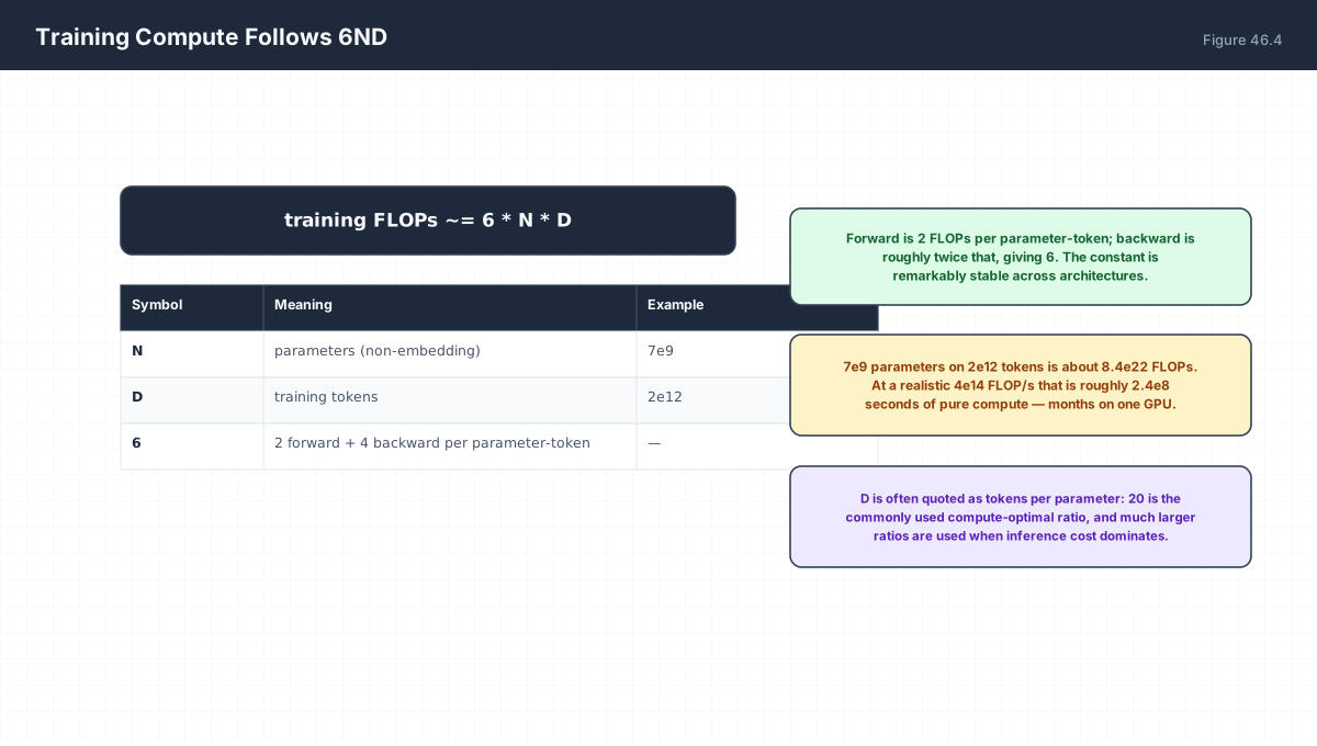
Forward pass: 2 FLOPs per parameter per token
             (one multiply, one add)

Backward pass: 4 FLOPs per parameter per token
             (gradient w.r.t. the weight, and w.r.t. the input)

Total: 6 N D  FLOPs, with N parameters and D tokens

This counts matmul work only. Attention's n^2 term and the
embedding lookup are separate, and the estimate gets less
accurate as sequence length grows.
def train_flops(n_params, n_tokens):
    return 6 * n_params * n_tokens

for n, d_tok in [(7e9, 2e12), (70e9, 2e12), (1.5e9, 3e11)]:
    f = train_flops(n, d_tok)
    gpu_days = f / 4e14 / 86400
    print(f"N={n:5.1e}  D={d_tok:5.1e}  FLOPs={f:8.2e}  ~{gpu_days:8.0f} GPU-days at 400 TFLOP/s")

print()
print("Chinchilla-style reference: ~20 tokens per parameter is")
print("compute-optimal when training cost is all that matters.")
for n, ratio in [(1.5e9, 20), (7e9, 20), (70e9, 20)]:
    print(f"  N={n:5.1e} -> D={n*ratio:5.1e} tokens")

print()
print("Inference dominates lifetime cost when D_infer >> D_train:")
print("  inference FLOPs per token ~= 2N, two orders below training")
print("  per token, but it runs billions of times.")
The formula is an estimate, not a law: it counts matmuls and ignores attention, which is quadratic in sequence length. For training at short context it is accurate enough to plan with; for long-context or inference-heavy analysis it is not.
6. Context Length
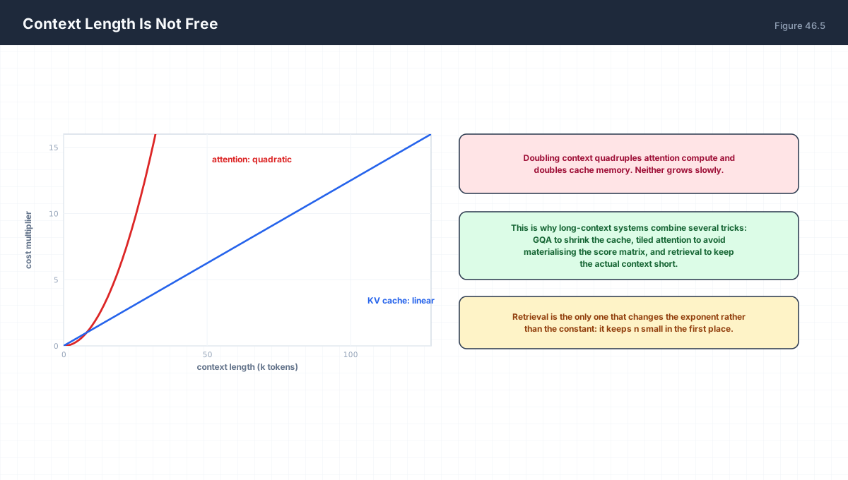
Two resources grow with context, at different rates:

  attention compute  O(n^2)   doubling context -> 4x compute
  KV cache memory    O(n)     doubling context -> 2x memory

Neither is free and neither is avoidable at the algorithm level.
Retrieval is the only approach that keeps n small instead of
making large n cheap.
for n in (2048, 8192, 32768, 131072):
    rel_attn = (n / 2048) ** 2
    rel_cache = n / 2048
    print(f"n={n:7d}  attention x{rel_attn:9.1f}  cache x{rel_cache:7.1f}")
Going from 2k to 128k context multiplies attention compute by 4096 and cache memory by 64. Any engineering effort spent on long context is an effort to attack one of those two numbers.
7. Worked Examples
7.1 Tokens per word
English averages roughly 1.3 tokens per word with a
modern BPE vocabulary. Code and non-Latin scripts are worse.
7.2 Vocabulary size trade-off
Larger vocab -> shorter sequences but a bigger embedding table
and a harder output softmax. 32k-128k is the practical range.
7.3 Weight tying
out = h @ E.T reuses the embedding matrix. Saves V*d parameters
and often improves quality, since input and output token
similarities are forced to agree.
7.4 Perplexity in practice
A model with perplexity 20 is as uncertain as a uniform
choice among 20 tokens. Vocabulary size affects the raw
number, so compare only within the same tokeniser.
7.5 Why 6ND ignores attention
The attention term is O(n^2 d) per layer; the parameter term is
O(N). At n = 2048 and d = 4096 they are comparable, which is
why the estimate drifts at long context.
8. Verify It in Python
import numpy as np

rng = np.random.default_rng(0)

# --- 1. embedding cost --------------------------------------
assert 128_000 * 4096 == 524_288_000
print(f"V=128k, d=4096 -> {128_000*4096:,} parameters")

# --- 2. weight tying halves the output head cost ------------
emb, head = 128_000 * 4096, 128_000 * 4096
assert emb + head == 2 * emb
print(f"tying saves {head:,} parameters")

# --- 3. lookup returns the row itself ------------------------
E = rng.normal(size=(1000, 16))
ids = np.array([3, 77, 512])
assert np.allclose(E[ids][1], E[77])
print("embedding lookup is a row selection")

# --- 4. gradient only touches used rows ---------------------
G = np.zeros_like(E)
G[ids] += 1.0
touched = int(np.count_nonzero(G.any(axis=1)))
assert touched == 3
print(f"a batch using 3 distinct ids updates {touched} of 1000 rows")

# --- 5. temperature reshapes the distribution ---------------
def softmax(z):
    e = np.exp(z - z.max())
    return e / e.sum()

logits = np.array([3.2, 2.4, 2.0, 1.2, 0.6, 0.1])
hot = softmax(logits / 2.0)
cold = softmax(logits / 0.5)
assert cold.max() > softmax(logits).max() > hot.max()
assert hot.min() > softmax(logits).min()
print(f"max prob: T=0.5 {cold.max():.4f} > T=1 {softmax(logits).max():.4f}"
      f" > T=2 {hot.max():.4f}")

# --- 6. entropy is monotone in temperature ------------------
def H(p):
    p = p[p > 0]
    return float(-(p * np.log(p)).sum())

ent = [H(softmax(logits / T)) for T in (0.25, 0.5, 1.0, 2.0, 10.0)]
assert all(a < b for a, b in zip(ent, ent[1:]))
print("entropy rises with temperature:", [round(e, 3) for e in ent])

# --- 7. top-k mass ------------------------------------------
p = softmax(logits)
order = np.argsort(p)[::-1]
assert np.isclose(p[order[:1]].sum(), p.max())
assert p[order[:len(p)]].sum() > 0.9999
print(f"top-1 keeps {p.max():.4f} of the mass")

# --- 8. 6ND arithmetic --------------------------------------
f = 6 * 7e9 * 2e12
assert np.isclose(f, 8.4e22)
print(f"7B params on 2T tokens = {f:.2e} FLOPs")

# --- 9. doubling tokens doubles training cost ---------------
assert np.isclose(6 * 1e9 * 2e12, 2 * (6 * 1e9 * 1e12))
print("training FLOPs are linear in tokens")

# --- 10. context cost grows quadratically -------------------
a, b = 2048, 4096
assert (b ** 2) / (a ** 2) == 4.0
assert b / a == 2.0
print("doubling context: 4x attention, 2x cache")
print("all assertions passed")
9. Practice Questions
- Why does subword tokenisation exist?
- Describe the BPE merge loop.
- Why are
mathandmathdifferent tokens? - Compute the embedding parameter count for V = 50,257, d = 768.
- What does weight tying save?
- Sketch the distribution at T = 0.5, 1.0 and 2.0.
- Contrast top-k with top-p.
- Derive the 6 in 6ND.
- When does the 6ND estimate become inaccurate?
- How do attention compute and KV cache scale differently with context?
10. Official References & Further Reading
Continue the Course
- Course Index: AI Mathematics Masterclass — All 48 Chapters
- Previous Chapter: Chapter 45: Generative Model Mathematics
- Next Chapter: Chapter 47: Numerical Stability, Precision & Underflow Mathematics
- Related Series: PyTorch Engineering Masterclass — All 16 Modules