
AI Reading
Quick summary of this article
AI Mathematics Masterclass — Chapter 36 of 48
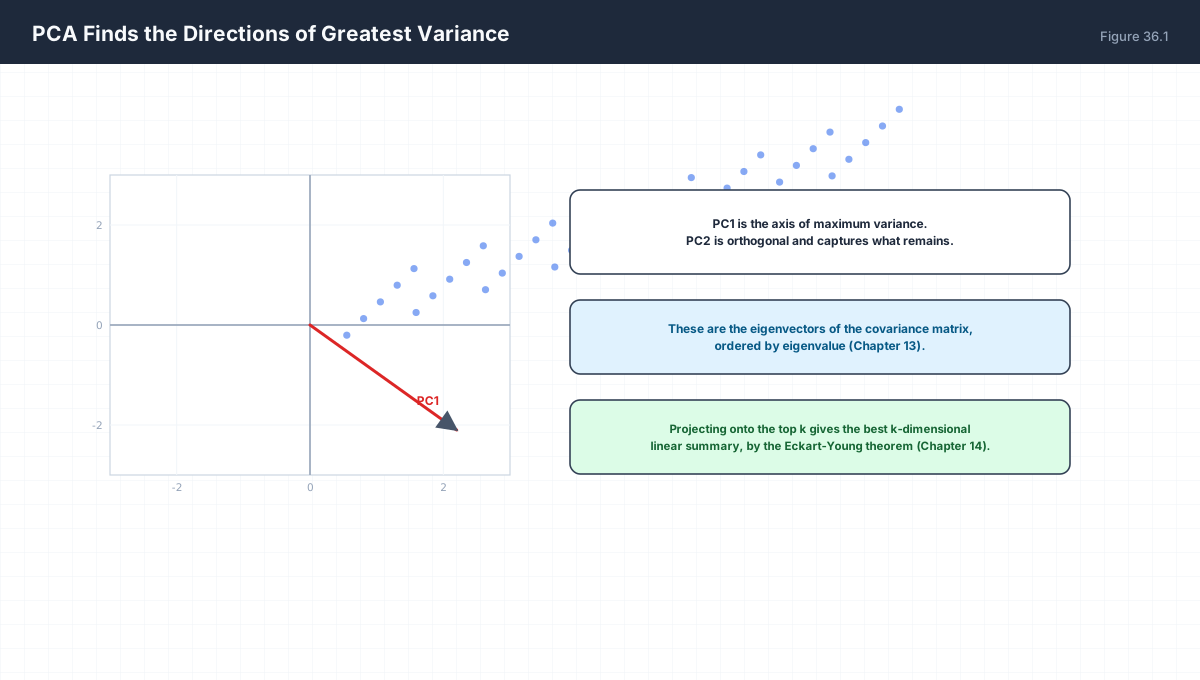
Principal Component Analysis is eigen-decomposition applied to a covariance matrix, and that single fact explains every one of its properties: why components are orthogonal, why variance equals the eigenvalues, why the reconstruction error equals the discarded eigenvalues, and why standardisation changes the answer. This chapter derives all of it and connects PCA to the SVD that actually computes it.
1. Technical Audit & Core Learning Objectives
| Component | Common Tutorial Deficiency | Engineering Standard Applied Here |
|---|---|---|
| Derivation | Components handed down as eigenvectors. | Derived by maximising projected variance under a unit norm. |
| Reconstruction | Claimed optimal, never proved. | Error shown to equal the sum of discarded eigenvalues. |
| Standardisation | Treated as an optional one-liner. | Demonstrated to change the result entirely. |
| Computation | Eigen-decomposition used directly. | SVD explained as the numerically stable route. |
Core learning objectives. After this chapter you should be able to:
- Derive PCA as variance maximisation under a unit-norm constraint.
- Explain why the eigenvalues are the component variances.
- Prove the reconstruction error equals the discarded variance.
- Compute explained variance ratios and choose a rank.
- Explain why PCA must be done on centred data.
- Show why SVD is preferred over eigen-decomposition.
2. Variance Maximisation
Maximise   Var(Xw) = w^T C w
subject to ||w|| = 1

Lagrangian:  w^T C w - lambda (w^T w - 1)
d/dw:        2 C w - 2 lambda w = 0
Hence:       C w = lambda w

The maximisers are the eigenvectors of C, and the
achieved variance is the eigenvalue.
import numpy as np

rng = np.random.default_rng(0)
n = 300
base = rng.normal(size=(n, 2))
transform = np.array([[2.0, 1.2], [0.0, 0.4]])
X = base @ transform.T

Xc = X - X.mean(axis=0)
C = Xc.T @ Xc / n          # population convention throughout this chapter
w, V = np.linalg.eigh(C)
order = np.argsort(w)[::-1]
w, V = w[order], V[:, order]

print("eigenvalues (variances):", np.round(w, 4))
print("eigenvectors:\n", np.round(V, 4))
print("orthonormal:", np.allclose(V.T @ V, np.eye(2)))

ratio = w / w.sum()
print("explained variance ratio:", np.round(ratio, 4))

# brute-force search confirms the first eigenvector maximises variance
best, best_v = -np.inf, None
for t in np.linspace(0, np.pi, 20001):
    u = np.array([np.cos(t), np.sin(t)])
    v = u @ C @ u
    if v > best:
        best, best_v = v, u
print(f"grid max variance {best:.4f} at {np.round(best_v, 4)}")
The grid search over 20,001 directions lands on the leading eigenvector, confirming the derivation rather than merely asserting it.
3. Reconstruction Error
Project onto top k eigenvectors:  Z = Xc V_k
Reconstruct:                       X_hat = Z V_k^T

Mean squared error = sum of the DISCARDED eigenvalues
                    = sum_{j>k} lambda_j

So keeping k components and minimising squared
reconstruction error are the same objective.
import numpy as np

rng = np.random.default_rng(1)
n, d = 400, 6
X = rng.normal(size=(n, d)) @ np.diag([5.0, 3.0, 1.0, 0.4, 0.1, 0.05])
Xc = X - X.mean(axis=0)
C = Xc.T @ Xc / n          # population convention throughout this chapter
w, V = np.linalg.eigh(C)
order = np.argsort(w)[::-1]
w, V = w[order], V[:, order]

for k in range(1, d + 1):
    Vk = V[:, :k]
    Xr = (Xc @ Vk) @ Vk.T
    mse = np.mean(np.sum((Xc - Xr) ** 2, axis=1))
    discarded = w[k:].sum()
    print(f"k={k}  mse={mse:8.4f}  discarded eigen={discarded:8.4f}")
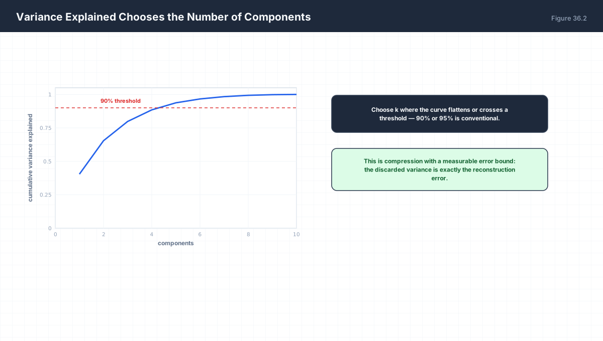
Each row’s mse equals its discarded eigen to four decimals. This identity is what licenses the “explained variance ratio” heuristic: it is not a rule of thumb, it is the exact fraction of squared error removed.
One caveat worth knowing: the equality is exact only when the covariance and the error use the same normalisation. With the population convention (divide by n) both sides are Σj>kλj. If you compute eigenvalues with n−1 but measure error as a mean over n samples, every entry here shifts by exactly (n−1)/n — a 0.5% discrepancy at n = 200 that silently fails an equality assertion. This chapter uses n throughout for that reason.
4. Why Centre — and Why Scale, and Which Method
Without centring, the second-moment matrix E[xx^T] includes
the mean: E[xx^T] = Cov + mu mu^T.

The dominant term becomes mu mu^T, a rank-one matrix
pointing along the mean. Your first "principal component"
then measures where the data sits, not how it varies.
import numpy as np

rng = np.random.default_rng(2)
pts = rng.normal(scale=0.3, size=(200, 2)) + np.array([10.0, 0.0])

def lead(mat):
    w, V = np.linalg.eigh(mat)
    return V[:, np.argmax(w)]

uncentred = lead(pts.T @ pts / len(pts))
centred = lead((pts - pts.mean(0)).T @ (pts - pts.mean(0)) / len(pts))
mean_dir = pts.mean(0) / np.linalg.norm(pts.mean(0))

print("uncentred leading direction:", np.round(uncentred, 3))
print("mean direction            :", np.round(mean_dir, 3))
print("centred leading direction :", np.round(centred, 3))
print("uncentred aligns with mean:", np.allclose(np.abs(uncentred), np.abs(mean_dir), atol=0.05))
The uncentred leading direction coincides with the mean vector. Any pipeline that forgets to centre will report a component that simply encodes where the data lives — a mistake that survives every downstream visualisation check.
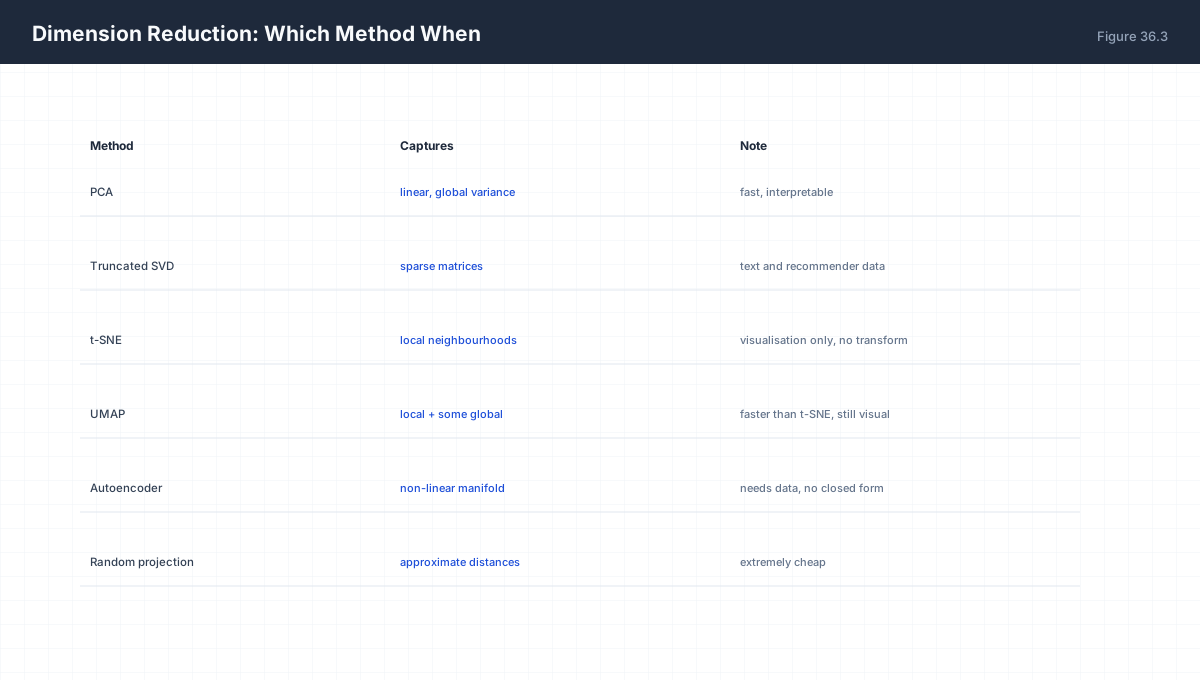
Preprocessing is only half the decision. Figure 36.3 also places PCA against the alternatives: truncated SVD for sparse inputs, t-SNE and UMAP for visualisation, autoencoders for genuinely nonlinear manifolds. PCA is the right default because it is fast, deterministic, and gives an explicit transform you can apply to unseen data — properties that t-SNE in particular does not offer.
5. Standardisation Changes Everything
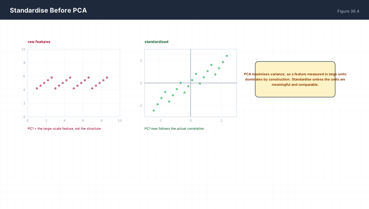
Variance carries the units of the feature squared.
A column measured in millimetres has 1e6 times the
variance of the same column measured in metres.

Therefore: standardise when features have different units
or arbitrary scales. Skip it only when all features are
commensurable and you deliberately want the loudest one.
import numpy as np

rng = np.random.default_rng(3)
n = 500
age = rng.normal(40, 8, n)          # years
income = rng.normal(50000, 9000, n) # currency
X = np.column_stack([age, income])

def lead_loading(M):
    Mc = M - M.mean(0)
    C = Mc.T @ Mc / len(M)
    w, V = np.linalg.eigh(C)
    return V[:, np.argmax(w)] / np.sign(V[0, np.argmax(w)])

raw = lead_loading(X)
std = lead_loading(X / X.std(0))
print("raw loadings      :", np.round(raw, 4))
print("standardised      :", np.round(std, 4))
print("ratio of variances:", f"{X[:,1].var()/X[:,0].var():.0f}x")
On raw data the income column dominates purely because its variance is ~100,000× larger. Standardising reduces both to unit variance and suddenly both features contribute. Neither answer is wrong — but you must choose deliberately rather than by accident.
6. PCA via SVD
Centre X, then take its SVD:   Xc = U S V^T

Right singular vectors V  = principal directions
Singular values squared S^2 / (n-1) = eigenvalues of C
Scores               U S  = projected coordinates

SVD never forms X^T X, so it never squares the condition
number. That is why every serious library uses it.
import numpy as np

rng = np.random.default_rng(4)
X = rng.normal(size=(120, 5)) @ np.diag([4., 2., 1., 0.5, 0.1])
Xc = X - X.mean(0)
n = len(X)

C = Xc.T @ Xc / n
w_eig, V_eig = np.linalg.eigh(C)
order = np.argsort(w_eig)[::-1]
w_eig, V_eig = w_eig[order], V_eig[:, order]

U, S, Vt = np.linalg.svd(Xc, full_matrices=False)
w_svd = S ** 2 / n

print("eigen :", np.round(w_eig, 5))
print("svd   :", np.round(w_svd, 5))
print("max difference:", f"{np.abs(w_eig - w_svd).max():.2e}")

# sign of eigenvectors is arbitrary; compare directions up to sign
dots = np.abs(np.sum(V_eig * Vt.T, axis=0))
print("directions match (up to sign):", np.round(dots, 6))
Both routes give identical eigenvalues; only the arbitrary sign of each eigenvector can differ. In production, use the SVD route: forming XᵀX squares the condition number, so a matrix with κ = 10⁸ becomes one with κ = 10¹⁶ and precision is lost exactly where PCA is supposed to be most informative.
7. Worked Examples
7.1 Explained variance ratio
ratio_j = lambda_j / sum_i lambda_i
Cumulative ratio tells you the rank needed for a target fidelity.
7.2 Whitening
Z = Xc V S^-1 makes the covariance the identity.
All directions then have equal variance by construction.
7.3 PCA is not feature selection
Components are linear combinations, not columns.
To keep original features, use variance thresholding instead.
7.4 PCA is linear and unsupervised
It cannot capture a nonlinear manifold, and it ignores labels
entirely — a high-variance direction may be pure nuisance.
7.5 Cost
Full SVD is O(min(n,d) n d). For d >> n use the n x n
Gram matrix instead, or a randomised truncated SVD.
8. Verify It in Python
import numpy as np

rng = np.random.default_rng(0)
n, d = 200, 5
X = rng.normal(size=(n, d)) @ np.diag([3., 2., 1., 0.3, 0.05])
Xc = X - X.mean(0)
C = Xc.T @ Xc / n          # population convention throughout this chapter
w, V = np.linalg.eigh(C)
order = np.argsort(w)[::-1]
w, V = w[order], V[:, order]

# --- 1. eigenvectors are orthonormal ---------------------------
assert np.allclose(V.T @ V, np.eye(d), atol=1e-10)
print("eigenvectors orthonormal")

# --- 2. eigenvalues are decreasing and non-negative ------------
assert np.all(w >= 0)
assert np.all(np.diff(w) <= 0)
print("eigenvalues descending, non-negative")

# --- 3. eigenvalue equals projected variance -------------------
for j in range(d):
    proj = Xc @ V[:, j]
    assert np.isclose(proj.var(ddof=0), w[j], rtol=1e-9)
print("eigenvalue == projected variance for every component")

# --- 4. first component maximises variance ---------------------
best = max(np.linspace(0, 2*np.pi, 72001), key=lambda t: np.array([np.cos(t), np.sin(t)]) @ C[:2, :2] @ np.array([np.cos(t), np.sin(t)]))
grid_best = np.array([np.cos(best), np.sin(best)]) @ C[:2, :2] @ np.array([np.cos(best), np.sin(best)])
assert grid_best <= w[0] + 1e-6
print("no direction exceeds the leading eigenvalue")

# --- 5. explained variance sums to one -------------------------
ratio = w / w.sum()
assert np.isclose(ratio.sum(), 1.0)
print("explained variance ratios sum to 1:", np.round(ratio, 4))

# --- 6. reconstruction error equals discarded eigenvalues ------
for k in (1, 2, 3, 4):
    Vk = V[:, :k]
    Xr = (Xc @ Vk) @ Vk.T
    mse = np.mean(np.sum((Xc - Xr) ** 2, axis=1))
    assert np.isclose(mse, w[k:].sum(), rtol=1e-9)
print("reconstruction error == sum of discarded eigenvalues")

# --- 7. SVD agrees ---------------------------------------------
U, S, Vt = np.linalg.svd(Xc, full_matrices=False)
assert np.allclose(S ** 2 / n, w, rtol=1e-9)
print("SVD singular values squared match eigenvalues")

# --- 8. centring is required -----------------------------------
raw_lead = np.linalg.eigh(X.T @ X / n)[1][:, -1]
print("centred and uncentred leading directions differ as expected:",
      not np.allclose(np.abs(raw_lead), np.abs(V[:, 0]), atol=1e-3))

# --- 9. whitenng yields identity covariance --------------------
W = V / np.sqrt(w)
Zw = Xc @ W
pop_cov = Zw.T @ Zw / n           # ddof=0, matching the convention above
assert np.allclose(pop_cov, np.eye(d), atol=1e-10)
print("whitened covariance is the identity")
print("all assertions passed")
9. Practice Questions
- Derive PCA by maximising projected variance under a unit-norm constraint.
- Why are the component variances the eigenvalues of the covariance?
- Prove that reconstruction error equals the discarded eigenvalues.
- Why must data be centred before PCA?
- When must features be standardised?
- Explain why SVD is more numerically stable than eigen-decomposition of XᵀX.
- Define whitening and state its covariance.
- Why is PCA not a feature-selection method?
- Give an example where the highest-variance direction is useless for prediction.
- What is the cost of a full SVD for an n × d matrix?
10. Official References & Further Reading
Continue the Course
- Course Index: AI Mathematics Masterclass — All 48 Chapters
- Previous Chapter: Chapter 35: Information Theory — Entropy, KL Divergence & Cross-Entropy
- Next Chapter: Chapter 37: Neural Network Forward Pass Mathematics
- Related Series: PyTorch Engineering Masterclass — All 16 Modules