
AI Reading
Quick summary of this article
AI Mathematics Masterclass — Chapter 2 of 48
Linear equations are the first mathematical structure a machine-learning practitioner meets and the last one they stop using. A forward pass is a system of linear equations; a least-squares fit is an over-determined system with no exact answer; a constrained optimisation problem is a system plus inequalities. This chapter builds the solver’s mental model: what a solution geometrically is, when it exists, why elimination finds it, and why a solver that is mathematically correct can still return catastrophic answers on a computer.
1. Technical Audit & Core Learning Objectives
Most treatments of linear equations present row-reduction as a mechanical procedure and stop. That produces students who can solve a 3×3 system by hand and cannot explain why their neural network’s normal equations returned NaN. This chapter keeps the mechanics but attaches each one to the failure mode it explains.
| Component | Common Tutorial Deficiency | Engineering Standard Applied Here |
|---|---|---|
| Solution geometry | “Solve for x” with no picture, so the three outcome cases feel arbitrary. | Each case drawn as an intersection of lines; inconsistency becomes visible, not memorised. |
| Elimination | Row operations listed as rules with no justification. | Operations shown to be invertible, therefore solution-preserving — the actual reason they are legal. |
| Numerics | Exact arithmetic assumed; conditioning and pivoting omitted. | Condition number introduced as the error-amplification factor, with a runnable demonstration. |
| Connection to ML | Never linked to models, so the topic seems like prerequisite theatre. | Every concept tied to a layer, a fitting problem, or a training-loop failure. |
Core learning objectives. After this chapter you should be able to:
- Read
a₁x + a₂y = bas a line, and a pair of them as their intersection. - Classify any system as having one, none, or infinitely many solutions from its row-echelon form.
- Perform Gaussian elimination with partial pivoting and explain why pivoting matters.
- Write a system in matrix form
Ax = band state the shapes ofA,x,b. - Compute a condition number and predict how much an input perturbation is amplified.
- Explain what
numpy.linalg.solveandlstsqdo differently, and when each applies.
2. A Single Equation Is a Line
The equation 2x + y = 4 does not have “an answer”. It has infinitely many answers — every point on a particular line. Rearranged as y = 4 − 2x, the structure is explicit: a slope of −2 and an intercept of 4.
That reframing is the entire geometric content of linear algebra: an equation is a constraint, and its solution set is a geometric object. One equation in two unknowns is a line. Two equations is the intersection of two lines — usually one point.
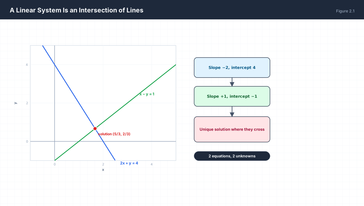
2x + y = 4      y = 4 − 2x      slope −2, intercept 4
x  − y = 1      y = x − 1       slope +1, intercept −1

Set them equal:   4 − 2x = x − 1
                  5 = 3x
                  x = 5/3 ≈ 1.667
                  y = 5/3 − 1 = 2/3 ≈ 0.667
In n dimensions the same logic holds with the objects renamed: one equation is a hyperplane of dimension n−1, and n independent hyperplanes pin down a single point. This is why a layer with n inputs and n outputs is invertible only when its weight matrix has n independent rows.
3. The Three Possible Outcomes
Two lines in a plane can meet once, never, or everywhere. There is no fourth option, and the same trichotomy governs systems of any size.
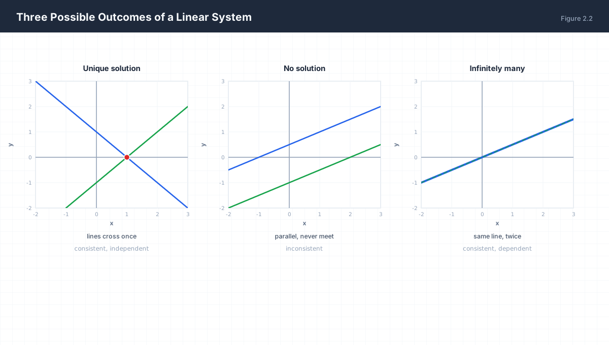
| Outcome | Geometry | Algebraic Signature | ML Consequence |
|---|---|---|---|
| Unique | Lines cross once | det(A) ≠ 0, full rank |
Layer is invertible; solve() succeeds |
| None | Parallel, distinct | Inconsistent; 0 = c with c ≠ 0 |
Over-determined fit — use least squares (Ch. 12) |
| Infinite | Same line twice | Rank < n; free variables exist | Under-determined; infinitely many valid weights |
The middle row deserves attention because it is the normal state of affairs in machine learning. You almost never have exactly as many equations as unknowns. With N training samples and d features, N ≫ d, so the system is inconsistent and no exact solution exists. That is not a bug — it is the reason least squares exists, and the reason gradient descent is used instead of a closed-form solve.
4. Gaussian Elimination
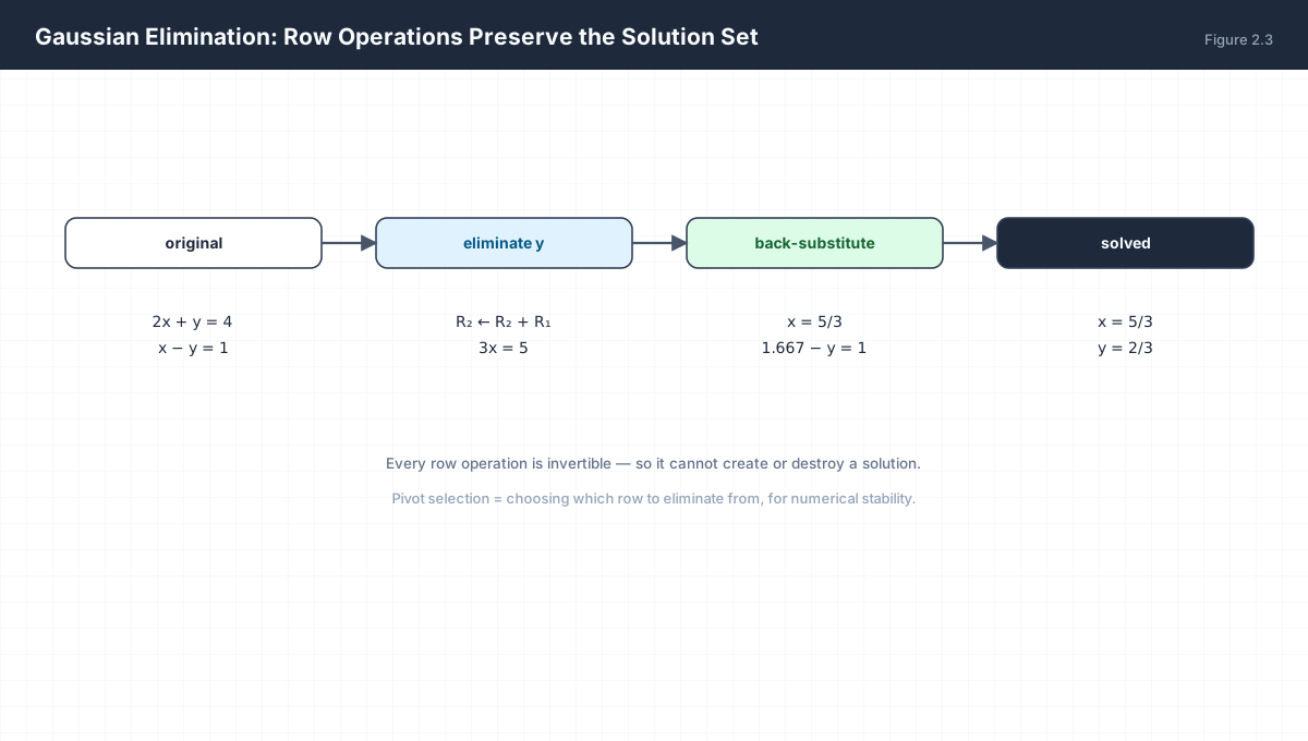
Elimination answers the question “how do I actually find the solution” without guessing. The idea is to combine equations so that one variable disappears, reducing an n×n system to an (n−1)×(n−1) system, repeatedly, until one equation has one unknown.
4.1 Why row operations are legal
Three operations preserve the solution set exactly, because each is invertible:
- Swap two rows. Invertible by swapping back.
- Multiply a row by a non-zero scalar. Invertible by dividing.
- Add a multiple of one row to another. Invertible by subtracting the same multiple.
Because each operation has an inverse, no information is created or destroyed. The set of points satisfying all equations is identical before and after. This is the property that lets a computer perform thousands of operations without drifting from the truth (in exact arithmetic — floating point is Section 6).
4.2 Forward elimination then back-substitution
import numpy as np

def gauss_solve(A, b):
    """Gaussian elimination with partial pivoting. Returns x."""
    A = A.astype(float).copy()
    b = b.astype(float).copy()
    n = len(b)
    for k in range(n):
        # partial pivoting: bring the largest |entry| in column k to the pivot
        p = k + int(np.argmax(np.abs(A[k:, k])))
        if abs(A[p, k]) < 1e-12:
            raise ValueError("matrix is singular")
        if p != k:
            A[[k, p]] = A[[p, k]]
            b[[k, p]] = b[[p, k]]
        for i in range(k + 1, n):
            f = A[i, k] / A[k, k]
            A[i, k:] -= f * A[k, k:]
            b[i] -= f * b[k]
    # back-substitution
    x = np.zeros(n)
    for i in range(n - 1, -1, -1):
        x[i] = (b[i] - A[i, i+1:] @ x[i+1:]) / A[i, i]
    return x

A = np.array([[2.0, 1.0], [1.0, -1.0]])
b = np.array([4.0, 1.0])
print(gauss_solve(A, b))          # [1.66666667 0.66666667]
print(np.linalg.solve(A, b))      # identical
The pivot loop is not decoration. Without it, dividing by a tiny pivot amplifies rounding error catastrophically — the numerical failure discussed in Section 6. np.linalg.solve uses LAPACK's getrf, which performs the same pivoting internally.
5. Matrix Form: Ax = b
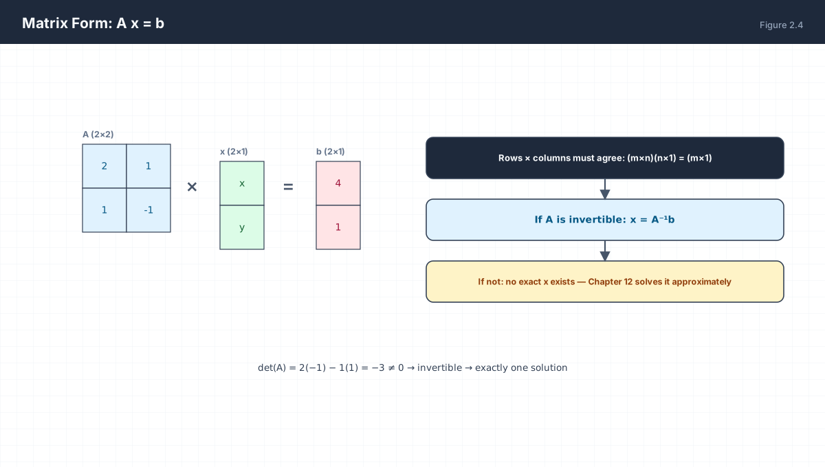
Writing the system as a matrix equation is what makes it computable at scale. The coefficients become a matrix, the unknowns a vector, and the right-hand side another vector.
import numpy as np

# Row picture: each row is one equation
A = np.array([[2.0, 1.0],
              [1.0, -1.0]])
b = np.array([4.0, 1.0])

# Shape rule: (m x n) @ (n,) -> (m,)
assert A.shape == (2, 2) and b.shape == (2,)
x = np.linalg.solve(A, b)
assert x.shape == (2,)
print("x =", x, " A@x =", A @ x)     # A@x reproduces b exactly

# Column picture: b is a combination of the columns of A
# b = x[0] * A[:,0] + x[1] * A[:,1]
rebuilt = x[0] * A[:, 0] + x[1] * A[:, 1]
print("column combination:", rebuilt)
The column picture is the more useful one for machine learning. It says: the output b is a weighted sum of the columns of A, with the weights being the unknowns. A linear layer does exactly this — the output is a combination of the columns of its weight matrix, and the input vector supplies the weights. If b cannot be expressed as such a combination, the system is inconsistent, which is Section 3's "no solution" case restated in the language of spans.
6. Conditioning: When a Correct Solver Gives a Wrong Answer
Every solver above is exact in real arithmetic. On a computer, inputs carry rounding error, and a system can amplify that error enormously.
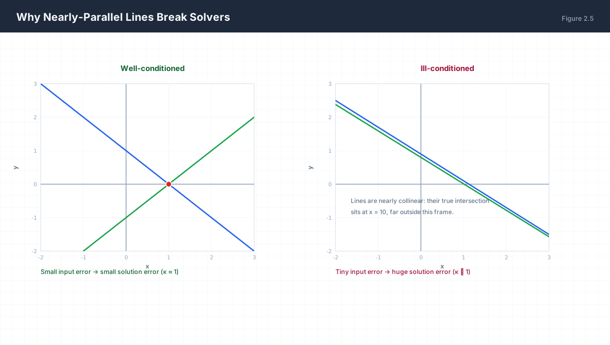
The condition number κ(A) bounds how much a relative error in b can grow in the solution:
‖Δx‖ / ‖x‖   ≤   κ(A) · ‖Δb‖ / ‖b‖

κ(A) = ‖A‖ · ‖A⁻¹‖          (2-norm: ratio of largest to smallest singular value)

κ ≈ 1        →  errors are not amplified  (well-conditioned)
κ = 10^k     →  you lose about k decimal digits of accuracy
import numpy as np

good = np.array([[1.0, 0.0], [0.0, 1.0]])          # perpendicular
bad  = np.array([[1.0, 1.0], [1.0, 1.0001]])       # nearly collinear rows

print("kappa(good) =", np.linalg.cond(good))       # 1.0
print("kappa(bad)  =", np.linalg.cond(bad))        # ~40000

b = np.array([2.0, 2.0])
x_clean = np.linalg.solve(bad, b)
x_pert  = np.linalg.solve(bad, b + np.array([0.0, 1e-4]))   # tiny perturbation
print("clean :", x_clean)
print("pert  :", x_pert)                                     # wildly different
print("relative change:", np.linalg.norm(x_pert - x_clean) / np.linalg.norm(x_clean))
This is why feature scaling precedes almost every classical model. Two features on wildly different magnitudes make columns of the design matrix nearly collinear, κ explodes, and the fitted coefficients become unstable — flipping sign when a single sample changes. Standardising features is not cosmetic; it is conditioning the system.
7. What the Solvers Actually Do
| Function | Requires | Method | Cost |
|---|---|---|---|
linalg.solve |
Square, non-singular A |
LU with partial pivoting | O(n³) |
linalg.lstsq |
Any shape, possibly inconsistent | SVD-based minimum-norm solution | O(mn²) |
linalg.inv(A) @ b |
Same as solve |
Explicit inverse — avoid | O(n³) + worse accuracy |
Never compute inv(A) @ b. Forming the inverse performs more floating-point operations than solving directly and loses accuracy, because the inverse itself may be far more ill-conditioned than A. The inverse is a mathematical object for analysis, not a computational step.
8. Worked Examples
8.1 Solving a 2×2 system exactly
3x + 2y = 12
 x −  y =  1

From the second: x = y + 1
Substitute:     3(y + 1) + 2y = 12
                5y = 9  →  y = 1.8
                x = 2.8

Check: 3(2.8) + 2(1.8) = 8.4 + 3.6 = 12 ✓
8.2 Detecting inconsistency
x + 2y = 3
2x + 4y = 7

Eliminate: R₂ ← R₂ − 2R₁  →  0 = 1     (contradiction)

Row 2 is exactly 2 × row 1 in the coefficients but not in the constant:
the left sides are proportional, the right sides are not → parallel lines.
8.3 Detecting infinite solutions
x + 2y = 3
2x + 4y = 6

R₂ ← R₂ − 2R₁  →  0 = 0     (tautology)

Row 2 is exactly 2 × row 1. Only one independent equation remains,
so y is free and x = 3 − 2y for any y. A one-parameter family.
8.4 Why a network's normal equations fail
Fitting y = Xw by least squares solves XᵀX w = Xᵀy. If two features are exact duplicates, XᵀX is singular and solve raises LinAlgError. The fix is either to drop a column or to use lstsq, which returns the minimum-norm solution instead of failing.
import numpy as np

X = np.array([[1.0, 1.0], [2.0, 2.0], [3.0, 3.0]])   # duplicated columns
y = np.array([1.0, 2.0, 3.0])

print("det(XtX) =", np.linalg.det(X.T @ X))          # 0.0
try:
    np.linalg.solve(X.T @ X, X.T @ y)
except np.linalg.LinAlgError as exc:
    print("solve failed:", exc)

w, *_ = np.linalg.lstsq(X, y, rcond=None)             # succeeds
print("minimum-norm w =", w, "sum =", w.sum())        # weights split evenly
9. Verify It in Python
Run this to confirm every claim in the chapter: the shape rule, the trichotomy, the conditioning effect, and the least-squares fallback.
import numpy as np

# --- 1. Shape rule -------------------------------------------------
A = np.array([[2.0, 1.0], [1.0, -1.0]])
b = np.array([4.0, 1.0])
x = np.linalg.solve(A, b)
assert np.allclose(A @ x, b)
assert abs(x[0] - 5 / 3) < 1e-12 and abs(x[1] - 2 / 3) < 1e-12
print("unique solution:", x)

# --- 2. Inconsistent system ----------------------------------------
A2 = np.array([[1.0, 2.0], [2.0, 4.0]])
print("det of linearly dependent matrix:", np.linalg.det(A2))   # 0.0

# --- 3. Condition numbers ------------------------------------------
good = np.eye(2)
bad = np.array([[1.0, 1.0], [1.0, 1.0001]])
print("kappa good/bad:", round(np.linalg.cond(good), 2),
      round(np.linalg.cond(bad), 1))
assert np.linalg.cond(bad) > 1000 * np.linalg.cond(good)

# --- 4. Perturbation amplification ---------------------------------
p = np.array([2.0, 2.0])
base = np.linalg.solve(bad, p)
shift = np.linalg.solve(bad, p + np.array([0.0, 1e-4]))
relative = np.linalg.norm(shift - base) / np.linalg.norm(base)
print(f"input change 5e-5 -> solution change {relative:.2e}")
assert relative > 0.1        # amplified by orders of magnitude

# --- 5. lstsq rescues the singular case ----------------------------
X = np.array([[1.0, 1.0], [2.0, 2.0], [3.0, 3.0]])
y = np.array([1.0, 2.0, 3.0])
w, *_ = np.linalg.lstsq(X, y, rcond=None)
print("min-norm weights:", w)
assert np.allclose(w, [0.5, 0.5])
print("all assertions passed")
10. Practice Questions
- Solve
4x − y = 7,x + 2y = 1and verify by substitution. - For which value of
kdoesx + ky = 2,2x + 4y = 5have no solution? Explain geometrically. - Why does multiplying a row by zero break the equivalence of the system, while multiplying by −1 does not?
- Given
κ(A) = 10⁶, roughly how many decimal digits of the solution are trustworthy in double precision? - Show that if
Ahas a zero row,det(A) = 0, and describe what that means for solvability. - Explain the column picture of
Ax = band why it makes "inconsistent" synonymous with "outside the span". - Construct a 3×3 system with infinitely many solutions and state its free variables.
- Why is
inv(A) @ bnumerically worse thansolve(A, b)even though both areO(n³)? - A design matrix has two features measured in metres and millimetres. Predict the effect on
κand on the fitted coefficients. - Under what condition does the normal-equation approach to linear regression fail outright, and what replaces it?
11. Official References & Further Reading
Continue the Course
- Course Index: AI Mathematics Masterclass — All 48 Chapters
- Previous Chapter: Chapter 1: Mathematics Foundations for AI
- Next Chapter: Chapter 3: Functions, Graphs & Transformations
- Related Series: PyTorch Engineering Masterclass — All 16 Modules