
AI Reading
Quick summary of this article
AI Mathematics Masterclass — Chapter 10 of 48
Matrix multiplication is the single operation that accounts for nearly all of the FLOPs in a modern neural network. It is also the operation whose shape rules generate the majority of runtime errors. This chapter covers the mechanics (row meets column), the transformation reading (matrices move space), the algebraic properties that are true and the ones that are not, and the practical consequence of associativity: the same product can cost 175× more depending on the order you choose.
1. Technical Audit & Core Learning Objectives
| Component | Common Tutorial Deficiency | Engineering Standard Applied Here |
|---|---|---|
| Mechanics | Formula given; no connection to the loop or the BLAS call. | Traced by hand on a 2×3 · 3×2 example, then matched to @. |
| Transformation | Abstraction stated but never shown acting on a shape. | Unit square drawn before and after four different matrices. |
| Properties | “Not commutative” asserted without consequence. | Non-commutativity shown numerically; associativity used for a cost argument. |
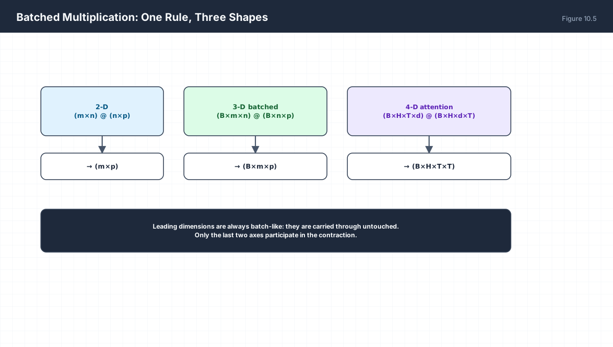
| Batching | Batch dimensions treated as an advanced topic. | One rule covering 2-D, 3-D, and 4-D attention shapes. |
Core learning objectives. After this chapter you should be able to:
- Compute a matrix product by hand and explain which index is summed.
- Predict the output shape of any multiplication, or identify it as invalid.
- Read a matrix as a linear transformation and state where basis vectors land.
- Show numerically that
AB ≠ BAbut(AB)C = A(BC). - Choose a multiplication order that reduces FLOPs.
- Extend the shape rule to batched and attention-shaped tensors.
2. Row Meets Column
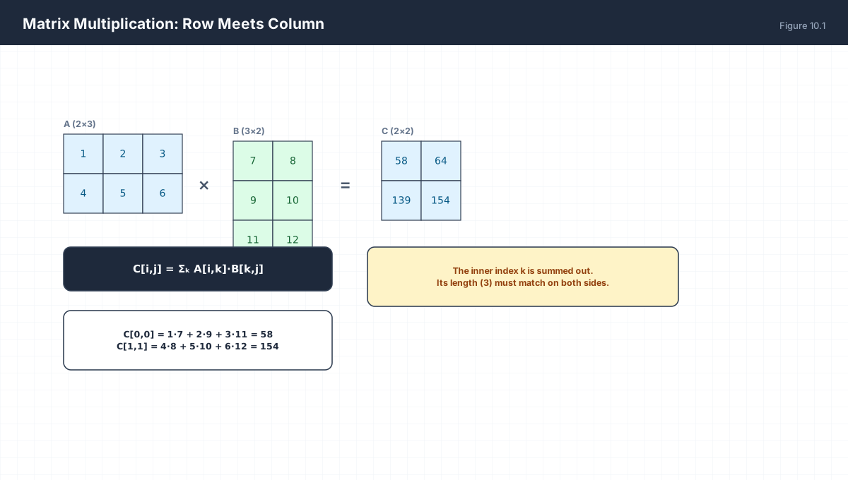
C = A @ B          A is (m×n), B is (n×p), C is (m×p)

C[i,j] = Σₖ A[i,k] · B[k,j]        k is summed out

C[0,0] = 1·7 + 2·9 + 3·11 = 58
C[1,1] = 4·8 + 5·10 + 6·12 = 154
The summed index k is the one that must have the same length on both sides. Everything else survives into the output. That single sentence is the entire shape rule.
3. The Shape Rule
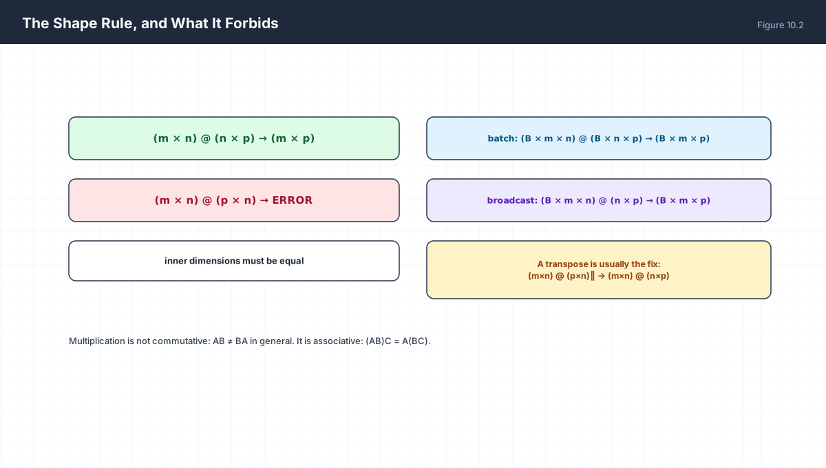
| Form | Rule | Example |
|---|---|---|
| matrix × matrix | (m×n)(n×p) → (m×p) | (3×4)(4×5) → (3×5) |
| matrix × vector | (m×n)(n,) → (m,) | (768×256)(256,) → (768,) |
| batched | (B×m×n)(B×n×p) → (B×m×p) | (8×32×64)(8×64×16) |
| broadcast | (B×m×n)(n×p) → (B×m×p) | same weight for every batch item |
import numpy as np

A = np.random.rand(3, 4)
B = np.random.rand(4, 5)
print((A @ B).shape)            # (3, 5)

try:
    A @ A
except ValueError as exc:
    print("invalid:", str(exc)[:60])

print((A @ A.T).shape)          # (3, 3) -- self-transpose makes the inner dims agree
4. A Matrix Moves Space
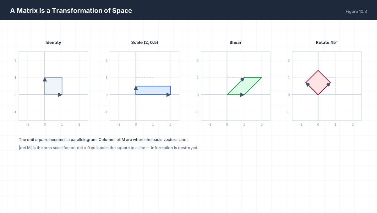
Multiplying by M on the left is a function. Its two most useful readings:
- Columns as destinations.
M @ e₁is the first column ofM. The matrix is completely determined by where it sends the basis vectors. - Determinant as area scale.
|det M|is the factor by which areas grow. Whendet M = 0, the square collapses to a line — the transformation has destroyed a dimension.
import numpy as np

sq = np.array([[0., 0.], [1., 0.], [1., 1.], [0., 1.]])

mats = {
    "identity": np.eye(2),
    "scale":    np.diag([2.0, 0.5]),
    "shear":    np.array([[1., 1.], [0., 1.]]),
    "rotate45": np.array([[0.7071, -0.7071], [0.7071, 0.7071]]),
    "singular": np.array([[1., 2.], [2., 4.]]),
}
for name, M in mats.items():
    print(f"{name:9s} det={np.linalg.det(M):+.3f}  e1 -> {np.round(M @ np.array([1., 0.]), 3)}")
The singular case is the informative one: det = 0, so the unit square maps onto a line segment. Two input directions now share an output direction, which is exactly the definition of M having a null space.
5. What Is and Is Not True
| Property | Holds? | Consequence |
|---|---|---|
AB = BA |
No | Rotation then shear ≠ shear then rotation |
(AB)C = A(BC) |
Yes | Free to reorder for cost |
A(B + C) = AB + AC |
Yes | Bias folding |
(AB)ᵀ = BᵀAᵀ |
Yes | Backpropagation’s workhorse |
AB = 0 ⇒ A=0 or B=0 |
No | Zero divisors exist; no cancellation |
import numpy as np

A = np.array([[0., 1.], [0., 0.]])      # nonzero, but A@A == 0
print("A @ A:\n", A @ A)
assert np.allclose(A @ A, 0)

R = np.array([[0., -1.], [1., 0.]])     # rotate 90
S = np.array([[1., 1.], [0., 1.]])      # shear
print("RS != SR:", not np.allclose(R @ S, S @ R))
print("associative:", np.allclose((A @ R) @ S, A @ (R @ S)))
Zero divisors matter in practice because they mean matrix multiplications have no cancellation law. A product of two non-zero weight matrices can be exactly zero — a silently dead pathway — and you cannot infer anything about the factors from that.
6. Batching and the Attention Shape
import numpy as np

B, H, T, d = 4, 8, 32, 64
Q = np.random.rand(B, H, T, d)
K = np.random.rand(B, H, T, d)

scores = Q @ K.swapaxes(-1, -2)          # (B,H,T,T)
print("attention scores:", scores.shape)

V = np.random.rand(B, H, T, d)
weights = np.random.rand(B, H, T)
weights /= weights.sum(axis=-1, keepdims=True)
out = weights[..., None, :] @ V          # (B,H,1,T) @ (B,H,T,d)
print("attention output:", out.shape)    # (B,H,1,d)
The swapaxes(-1, -2) is important: it says “transpose the last two axes”, leaving the batch axes alone. Writing K.T would reverse all four axes and produce nonsense. This is the practical reason to think in terms of leading versus trailing axes rather than in terms of a single transpose.
7. Worked Examples
7.1 By hand
A = [[1,2],[3,4]]   B = [[5,6],[7,8]]
C[0,0] = 1·5 + 2·7 = 19
C[0,1] = 1·6 + 2·8 = 22
C[1,0] = 3·5 + 4·7 = 43
C[1,1] = 3·6 + 4·8 = 50
C = [[19,22],[43,50]]
7.2 Identify invalid products
(2×3) @ (2×3)   invalid — inner 3 vs 2
(2×3) @ (3×2)   valid   → (2×2)
(2×3) @ (3,)    valid   → (2,)
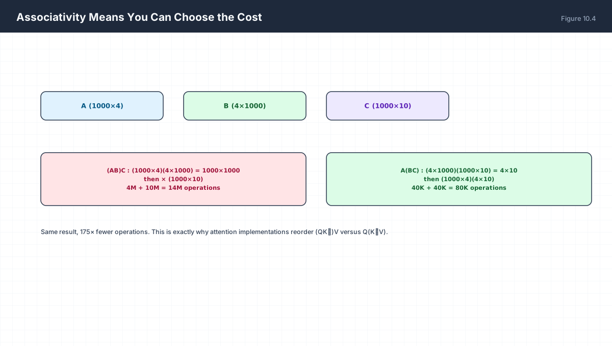
7.3 Cost of two orders
A(1000×4), B(4×1000), C(1000×10)

(AB)C: AB is 1000×1000 costing 4M mults, then × C costs 10M   → 14M
A(BC): BC is 4×10 costing 40K, then A × BC costs 40K          → 80K

80K / 14M ≈ 0.0057  →  175× cheaper
7.4 Where basis vectors land
M = [[2,0],[0,3]]
M @ e₁ = (2, 0)   first column
M @ e₂ = (0, 3)   second column
det = 6, so areas grow 6×
7.5 Bias folding
y = Wx + b  can be written  y = [W | b] @ [x; 1]
This is why a bias is an extra column, not a separate operation.
8. Verify It in Python
import numpy as np

# --- 1. hand-computed product -------------------------------------
A = np.array([[1., 2.], [3., 4.]])
B = np.array([[5., 6.], [7., 8.]])
assert np.allclose(A @ B, [[19., 22.], [43., 50.]])
print(A @ B)

# --- 2. shape rule and invalidity ---------------------------------
assert (np.zeros((2, 3)) @ np.zeros((3, 2))).shape == (2, 2)
try:
    np.zeros((2, 3)) @ np.zeros((2, 3))
    raise AssertionError("should not multiply")
except ValueError:
    print("invalid product rejected")

# --- 3. non-commutative but associative ---------------------------
R = np.array([[0., -1.], [1., 0.]])
S = np.array([[1., 1.], [0., 1.]])
assert not np.allclose(R @ S, S @ R)
assert np.allclose((R @ S) @ R, R @ (S @ R))
print("non-commutative, associative")

# --- 4. zero divisors exist --------------------------------------
Z = np.array([[0., 1.], [0., 0.]])
assert np.allclose(Z @ Z, 0) and not np.allclose(Z, 0)
print("nonzero matrix squared to zero")

# --- 5. columns are basis images ---------------------------------
M = np.diag([2.0, 3.0])
assert np.allclose(M @ np.array([1., 0.]), M[:, 0])
assert np.isclose(np.linalg.det(M), 6.0)
print("det:", np.linalg.det(M))

# --- 6. transposition reverses order -----------------------------
X = np.random.rand(2, 3); Y = np.random.rand(3, 4)
assert np.allclose((X @ Y).T, Y.T @ X.T)
print("(AB)T = BT AT")

# --- 7. batched attention shape ----------------------------------
Bs, Hs, Ts, ds = 2, 4, 16, 32
Q = np.random.rand(Bs, Hs, Ts, ds); K = np.random.rand(Bs, Hs, Ts, ds)
scores = Q @ K.swapaxes(-1, -2)
assert scores.shape == (Bs, Hs, Ts, Ts)
print("scores:", scores.shape)

# --- 8. associativity buys real savings --------------------------
a, b, c = np.random.rand(1000, 4), np.random.rand(4, 1000), np.random.rand(1000, 10)
assert np.allclose((a @ b) @ c, a @ (b @ c), atol=1e-8)
print("both orders agree to 1e-8")
print("all assertions passed")
9. Practice Questions
- Compute
[[1,2,3]] @ [[4],[5],[6]]and state its shape. - Which of these are valid:
(3×4)@(4×2),(3×4)@(3×2),(4,)@(4×2)? - Give two non-zero 2×2 matrices whose product is zero.
- Show numerically that rotation and shear do not commute.
- For
M = [[1,1],[0,1]], state wheree₁ande₂land and the determinant. - Compute the FLOP ratio for
(A(500×2))(B(2×500))(C(500×3))in both orders. - Explain why
K.Tis wrong for a 4-D attention tensor and what to use instead. - Write
y = Wx + bas a single matrix product. - Why does
det M = 0imply information is destroyed? - Give the shape of
W ∈ nn.Linear(64, 16)weight and the output shape for a batch of 8.
10. Official References & Further Reading
Continue the Course
- Course Index: AI Mathematics Masterclass — All 48 Chapters
- Previous Chapter: Chapter 9: Matrices & Matrix Operations
- Next Chapter: Chapter 11: Norms, Distances & Similarity Measures
- Related Series: PyTorch Engineering Masterclass — All 16 Modules