
AI Reading
Quick summary of this article
AI Mathematics Masterclass — Chapter 21 of 48
Backpropagation is the chain rule applied to a composition graph, evaluated from the output backwards. That is the whole idea, and it fits in one identity: the gradient passed to a node is its local derivative multiplied by the gradient coming from above. This chapter derives that identity, applies it to a real network layer by layer, implements a miniature autograd engine, and then explains the two failure modes — vanishing and exploding gradients — as arithmetic consequences of multiplying many factors together.
1. Technical Audit & Core Learning Objectives
| Component | Common Tutorial Deficiency | Engineering Standard Applied Here |
|---|---|---|
| Chain rule | Stated for two functions and never extended to a graph. | Extended to arbitrary depth, then to a branching graph. |
| Backprop | Described as a “special algorithm”. | Shown to be one identity applied at each node, in reverse. |
| Implementation | Deferred entirely to the framework. | A working 40-line autograd engine is built and checked. |
| Pathologies | Vanishing gradients asserted. | Measured across depth, with the fix for each. |
Core learning objectives. After this chapter you should be able to:
- Apply the chain rule through a chain of four functions.
- State the local-times-upstream identity for gradient flow.
- Derive gradients for a two-layer network by hand.
- Implement a minimal reverse-mode autograd engine.
- Verify analytic gradients against finite differences.
- Quantify gradient decay across depth and name the remedies.
2. The Chain Rule Along a Path
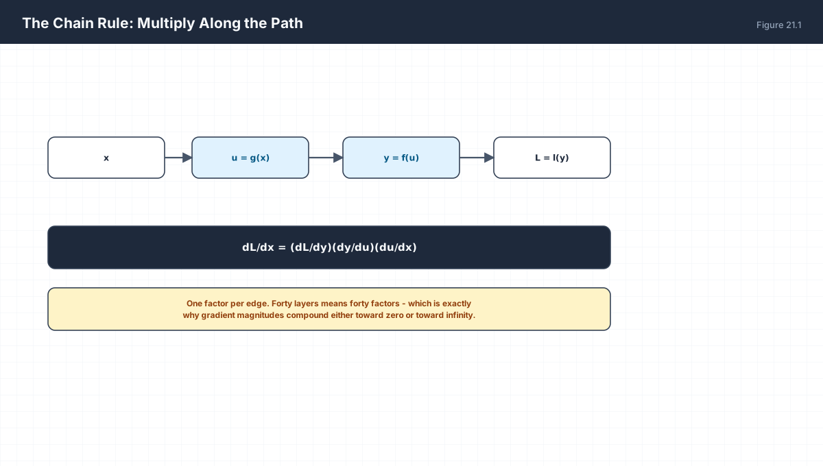
L = l(f(g(x)))

dL/dx = (dL/dl)(dl/df)(df/dg)(dg/dx)

Read right to left: the derivative of the innermost function
comes last. Read as a product: any factor near zero kills
the whole product; any factor above one inflates it.
import numpy as np

g = lambda x: 2 * x + 1
f = lambda u: u ** 2
l = lambda y: np.log(y)

x0 = 1.0
# dL/dx = (1/y) * (2u) * 2   with u = g(x0), y = f(u)
u0, y0 = g(x0), f(g(x0))
dL_dx = (1 / y0) * (2 * u0) * 2
print("analytic:", dL_dx)

composed = lambda x: l(f(g(x)))
h = 1e-7
numeric = (composed(x0 + h) - composed(x0 - h)) / (2 * h)
print("numeric :", round(numeric, 8))
assert np.isclose(dL_dx, numeric, atol=1e-5)
3. Backpropagation Is Reverse Traversal
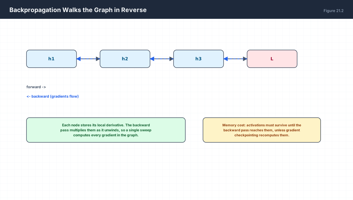
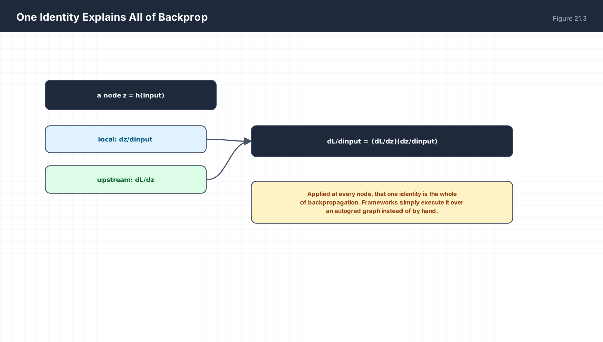
For a node computing z from its inputs:

  gradient passed to input = (dL/dz) * (dz/dinput)
                             ^upstream   ^local

At the loss, dL/dz = 1 (seed).
At each node, multiply. Where paths merge, add.
import numpy as np

def numerical_grad(fn, p, h=1e-6):
    g = np.zeros_like(p, dtype=float)
    for i in range(p.size):
        e = np.zeros_like(p, dtype=float); e[i] = h
        g[i] = (fn(p + e) - fn(p - e)) / (2 * h)
    return g

def relu(t):
    return np.maximum(0.0, t)

def net(params, x):
    W1, b1, W2, b2 = params
    h = relu(x @ W1 + b1)
    return np.sum(h @ W2 + b2)

rng = np.random.default_rng(0)
W1 = rng.normal(size=(3, 4)) * 0.5
b1 = np.zeros(4)
W2 = rng.normal(size=(4, 1)) * 0.5
b2 = np.zeros(1)
x = rng.normal(size=(2, 3))

def flat(W1, b1, W2, b2):
    return np.concatenate([W1.ravel(), b1, W2.ravel(), b2])

def unflat(p):
    W1 = p[0:12].reshape(3, 4); b1 = p[12:16]
    W2 = p[16:20].reshape(4, 1); b2 = p[20:21]
    return W1, b1, W2, b2

p0 = flat(W1, b1, W2, b2)
g = numerical_grad(lambda p: net(unflat(p), x), p0)
print("finite-difference gradient norm:", round(np.linalg.norm(g), 6))
print("nonzero entries:", int(np.sum(np.abs(g) > 1e-8)))
4. A Minimal Autograd Engine
Reverse-mode differentiation is not complicated machinery. It is a recording of the forward operations, each storing its local derivative, plus a reverse sweep that multiplies. This is a complete implementation:
import numpy as np

class Val:
    """A scalar with a gradient, recording the op that produced it."""
    def __init__(self, data, parents=(), local=()):
        self.data = float(data)
        self.grad = 0.0
        self.parents = parents
        self.local = local          # d(self)/d(parent) for each parent

    def __add__(self, other):
        other = other if isinstance(other, Val) else Val(other)
        return Val(self.data + other.data, (self, other), (1.0, 1.0))

    def __mul__(self, other):
        other = other if isinstance(other, Val) else Val(other)
        return Val(self.data * other.data, (self, other), (other.data, self.data))

    def __pow__(self, n):
        return Val(self.data ** n, (self,), (n * self.data ** (n - 1),))

    def tanh(self):
        t = np.tanh(self.data)
        return Val(t, (self,), (1 - t ** 2,))

    def backward(self):
        order, seen = [], set()
        def topo(v):
            if id(v) in seen:
                return
            seen.add(id(v))
            for p_ in v.parents:
                topo(p_)
            order.append(v)
        topo(self)
        self.grad = 1.0
        for v in reversed(order):
            for p_, d in zip(v.parents, v.local):
                p_.grad += v.grad * d

a, b = Val(2.0), Val(-3.0)
out = a * b + b ** 2 + (a * 3.0).tanh()
out.backward()
print(f"out={out.data:.6f}  da={a.grad:.6f}  db={b.grad:.6f}")

# check against finite differences
def f(a_, b_):
    return a_ * b_ + b_ ** 2 + np.tanh(a_ * 3.0)
h = 1e-6
print("numeric da:", round((f(2+h, -3) - f(2-h, -3)) / (2*h), 6))
print("numeric db:", round((f(2, -3+h) - f(2, -3-h)) / (2*h), 6))
Forty lines, and it reproduces what a framework does. The only additions in production are tensor data instead of scalars, and the topological sort applied to a much larger graph. The identity it implements is exactly the one in Figure 21.3.
5. Gradient Flow Across Depth
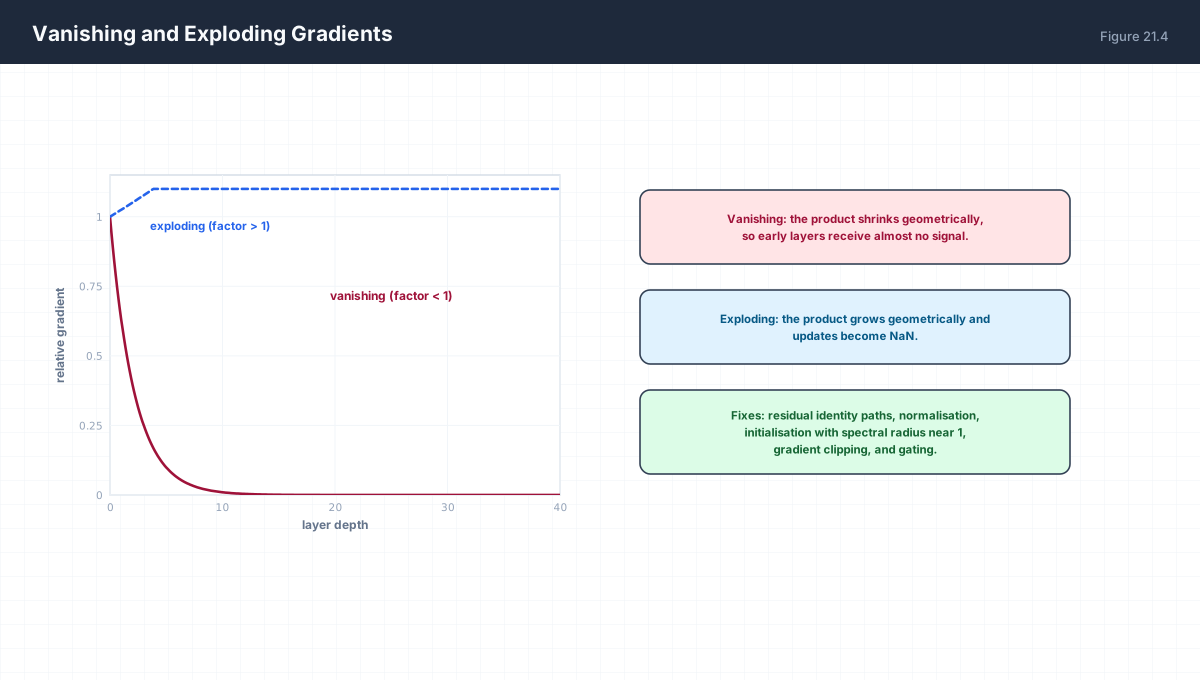
import numpy as np

for factor, name in ((0.25, "sigmoid"), (0.9, "mild"), (1.1, "slightly >1")):
    print(f"{name:12s} 10 layers={factor**10:.3e}  30 layers={factor**30:.3e}")

# a deep chain with sigmoid saturating
def chain_gradient(depth, sigma):
    return np.prod([sigma] * depth)

print("\nsigmoid at saturation (derivative 0.01):")
for d in (5, 20, 50):
    print(f"  depth {d:2d}: {chain_gradient(d, 0.01):.2e}")
| Failure | Cause | Remedy |
|---|---|---|
| Vanishing | Each factor < 1 (saturated sigmoid, small weights) | Residual paths, ReLU, LayerNorm, ρ ≈ 1 init |
| Exploding | Each factor > 1 (large weights, unstable recurrence) | Gradient clipping, spectral normalisation, smaller init |
| Dead units | ReLU stuck at zero → local derivative exactly 0 | Leaky ReLU, GELU, lower learning rate |
6. Worked Examples
6.1 Three-link chain
y = (3x + 2)^2,  x = 1
dy/dx = 2(3x+2)·3 = 6(3x+2)
At x=1: 6·5 = 30
6.2 Two-layer network gradient
h = xW1 + b1
y = hW2
L = (y - t)^2

dL/dy = 2(y - t)
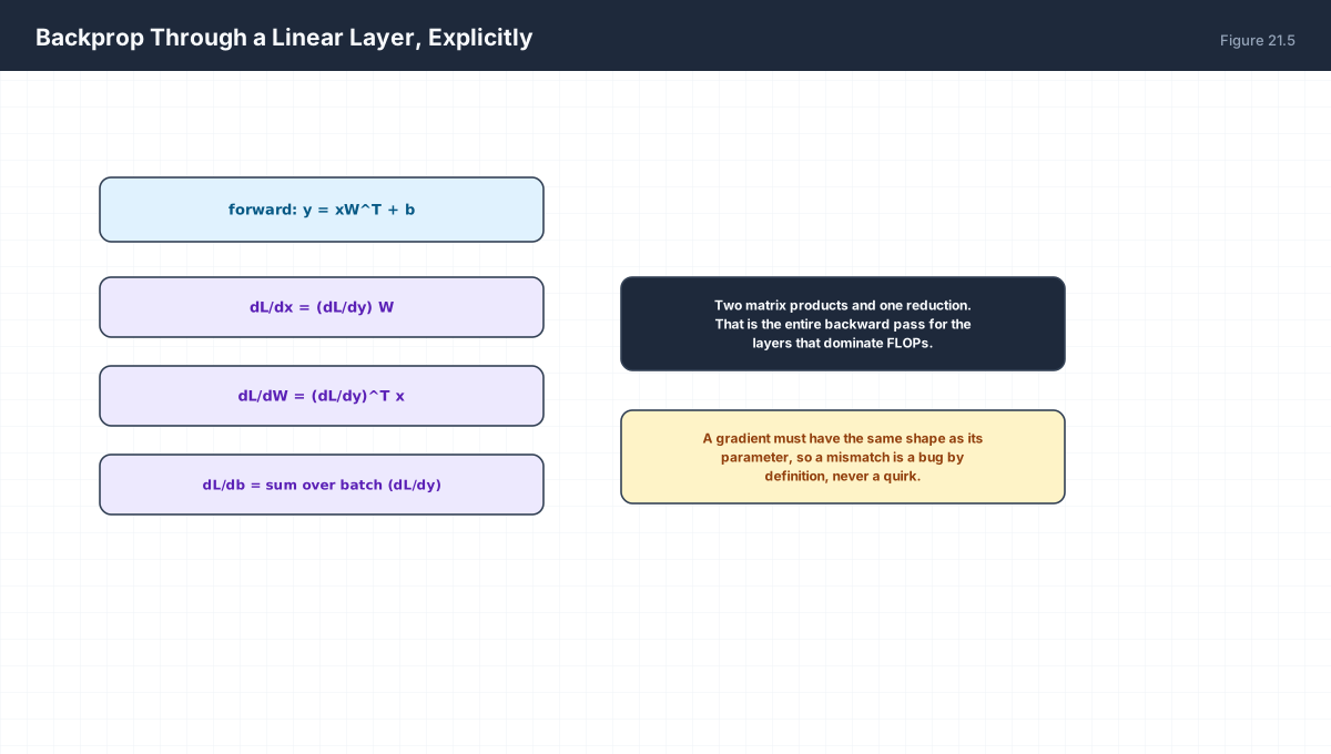
dL/dW2 = h^T (dL/dy)
dL/dh = (dL/dy) W2^T
dL/dW1 = x^T (dL/dh)
6.3 Gradient through softmax plus cross-entropy
For one-hot targets, the two Jacobians cancel to:
  dL/dz = p - onehot(y)
A surprisingly clean result, and a common interview question.
6.4 Why a shared weight gets a summed gradient
y1 = w·x1,  y2 = w·x2,  L = y1 + y2
dL/dw = x1 + x2
Two paths through w, so two contributions added.
6.5 Residual gradient
y = x + f(x)
dy/dx = 1 + f'(x)
The identity term guarantees a gradient of at least 1 reaches
earlier layers, regardless of how small f' becomes.
7. Verify It in Python
import numpy as np

def nd(f, x, h=1e-6):
    return (f(x + h) - f(x - h)) / (2 * h)

# --- 1. chain rule through four functions -------------------------
g = lambda x: 2 * x + 1
f = lambda u: u ** 2
ell = lambda y: np.log(y)
composed = lambda x: ell(f(g(x)))
x0 = 1.5
analytic = (1 / f(g(x0))) * (2 * g(x0)) * 2
assert np.isclose(analytic, nd(composed, x0), atol=1e-5)
print("chain rule verified:", round(analytic, 6))

# --- 2. linear layer gradients match finite differences -----------
rng = np.random.default_rng(1)
X = rng.normal(size=(4, 3))
W = rng.normal(size=(3, 2))
b = rng.normal(size=2)
t = rng.normal(size=(4, 2))

def loss(W_, b_):
    return np.sum((X @ W_ + b_ - t) ** 2)

dL_dy = 2 * (X @ W + b - t)
dW = X.T @ dL_dy
db = dL_dy.sum(axis=0)

# numeric check on a few entries
for i, j in [(0, 0), (2, 1)]:
    Wp, Wm = W.copy(), W.copy()
    Wp[i, j] += 1e-6; Wm[i, j] -= 1e-6
    num = (loss(Wp, b) - loss(Wm, b)) / (2e-6)
    assert np.isclose(dW[i, j], num, atol=1e-4)
print("dW entries verified numerically")

for j in range(2):
    bp, bm = b.copy(), b.copy()
    bp[j] += 1e-6; bm[j] -= 1e-6
    num = (loss(W, bp) - loss(W, bm)) / (2e-6)
    assert np.isclose(db[j], num, atol=1e-4)
print("db verified numerically")

# --- 3. gradient of softmax + cross-entropy -----------------------
def softmax(z):
    z = z - z.max(axis=-1, keepdims=True)
    e = np.exp(z)
    return e / e.sum(axis=-1, keepdims=True)

z = rng.normal(size=(3, 5))
labels = np.array([0, 2, 4])
onehot = np.zeros_like(z)
onehot[np.arange(3), labels] = 1.0
grad = softmax(z) - onehot                     # p - y
assert grad.shape == z.shape
assert np.allclose(grad.sum(axis=-1), 0.0)     # each row sums to zero
print("softmax+CE gradient is p - onehot, rows sum to 0")

# --- 4. shared weight gradient is summed -------------------------
def two_path(w):
    w = float(np.asarray(w).ravel()[0])
    return w * 2.0 + w * 5.0
assert np.isclose(float(nd(two_path, np.array([1.0]))), 7.0)
print("shared weight gradient sums both paths: 2 + 5 = 7")

# --- 5. residual preserves gradient magnitude --------------------
seq = lambda x: 0.001 * x            # almost-zero local derivative
res = lambda x: x + 0.001 * x        # with identity path
assert nd(seq, 1.0) < 0.01
assert np.isclose(nd(res, 1.0), 1.001)
print("residual keeps total gradient near 1")

# --- 6. vanishing gradient magnitude across depth ----------------
factors = [0.25] * 20
assert np.prod(factors) < 1e-12
print("20 sigmoid factors:", f"{np.prod(factors):.2e}")

# --- 7. gradient clipping bounds the update ---------------------
gradient = np.array([30.0, 40.0])
norm = np.linalg.norm(gradient)
clipped = gradient * min(1.0, 1.0 / norm)
assert np.isclose(np.linalg.norm(clipped), 1.0)
print("clipped gradient norm:", np.linalg.norm(clipped))
print("all assertions passed")
8. Practice Questions
- Apply the chain rule to
y = (3x + 2)²and evaluate atx = 1. - State the local-times-upstream identity in your own words.
- Why does the backward pass start with
dL/dL = 1? - Derive
dL/dW1for a two-layer network with a squared loss. - Show that
dL/dz = p − onehot(y)for softmax plus cross-entropy. - Why is the gradient of a twice-used weight a sum of two terms?
- Explain why
y = x + f(x)bounds gradient decay from below. - Compute
0.25²⁰and state its implication for a 20-layer sigmoid network. - Name three remedies for exploding gradients.
- Why does the topological sort matter in a general graph?
9. Official References & Further Reading
Continue the Course
- Course Index: AI Mathematics Masterclass — All 48 Chapters
- Previous Chapter: Chapter 20: Partial Derivatives & Gradients
- Next Chapter: Chapter 22: Jacobians, Hessians & Second-Order Geometry
- Related Series: PyTorch Engineering Masterclass — All 16 Modules