
AI Reading
Quick summary of this article
AI Mathematics Masterclass — Chapter 8 of 48
Five operations cover almost every vector computation in a neural network: addition, scalar multiplication, the three norms, and the dot product. The dot product is the important one — it is simultaneously a classifier logit, a retrieval similarity, and a neuron’s pre-activation. This chapter derives it geometrically, shows why cosine similarity is the dot product with magnitude divided out, and demonstrates the one numerical property that matters: the dot product amplifies its inputs, so its scale grows with dimension.
1. Technical Audit & Core Learning Objectives
Vector operations are usually demonstrated with arrows and then left behind. What is missing is the connection between the algebra and the failures practitioners see: unbounded logits, similarity scores that depend on text length, and gradient norms that explode with depth.
| Component | Common Tutorial Deficiency | Engineering Standard Applied Here |
|---|---|---|
| Addition / scaling | Drawn as arrows, never linked to residuals or attention blending. | Geometric rules connected to actual architectural operations. |
| Norms | Only the L2 norm is taught; L1 and L∞ treated as trivia. | All three with the regularisation each one induces. |
| Dot product | Given as a formula with no geometric content. | Derived as a projection, then shown as the shape every logit takes. |
| Scale | Dot-product magnitude growth with dimension never mentioned. | Explained as the reason attention divides by √d. |
Core learning objectives. After this chapter you should be able to:
- Add and scale vectors geometrically and componentwise.
- Compute L1, L2, and L∞ norms and state which regulariser each corresponds to.
- Compute a dot product, a projection, and an angle between two vectors.
- Explain the sign of the dot product in terms of the angle.
- Derive the attention scaling factor √d from variance growth.
- Recognise the dot product inside a logit, a similarity score, and a weighted sum.
2. Addition and Scaling
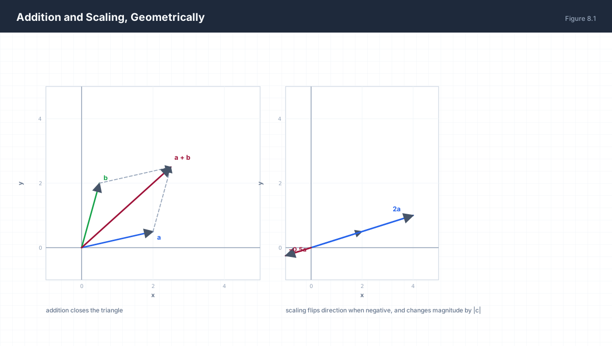
u + v = (u₁+v₁, u₂+v₂, …, uₙ+vₙ)     componentwise
c·u   = (c·u₁,  c·u₂,  …, c·uₙ)      componentwise

Commutative:  u + v = v + u
Associative:  (u+v)+w = u+(v+w)
Distributive: c(u+v) = cu + cv
Addition is the operation behind residual connections — x + f(x) adds two vectors of identical shape — and behind attention output, which is a weighted sum of value vectors. Scaling appears in learning-rate application, in gradient clipping, and in the temperature parameter of sampling.
3. The Three Norms
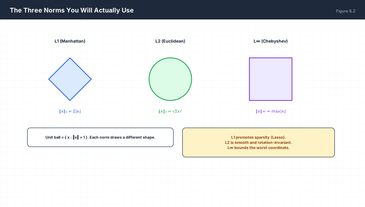
| Norm | Formula | Induced Regulariser | Effect |
|---|---|---|---|
| L1 | Σ|xᵢ| |
Lasso | Drives weights exactly to zero — sparsity |
| L2 | √Σxᵢ² |
Ridge / weight decay | Shrinks all weights smoothly |
| L∞ | max|xᵢ| |
Adversarial robustness (ε-ball) | Bounds the single worst coordinate |
import numpy as np

x = np.array([3.0, -4.0, 0.0])
print("L1 :", np.linalg.norm(x, 1))        # 7.0
print("L2 :", np.linalg.norm(x, 2))        # 5.0
print("Linf:", np.linalg.norm(x, np.inf))  # 4.0

# gradient clipping uses the L2 norm
g = np.array([10.0, 0.0, 0.0])
clip = 1.0
scaled = g * min(1.0, clip / np.linalg.norm(g))
print("clipped norm:", np.linalg.norm(scaled))   # 1.0
The shapes in Figure 8.2 explain the regularisation behaviour directly. The L1 ball has corners on the axes, so the optimum of a constrained problem tends to land exactly on a corner — where one coordinate is zero. The L2 ball is smooth, so the optimum lands somewhere on the curve with all coordinates non-zero. That single geometric fact is the whole difference between Lasso sparsity and Ridge shrinkage.
4. The Dot Product
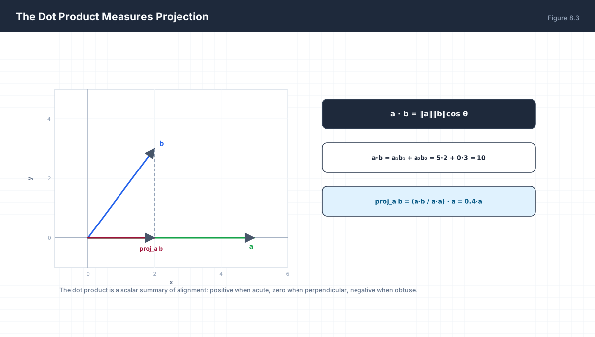
a · b = Σᵢ aᵢbᵢ = ‖a‖ ‖b‖ cos θ

Equivalent readings:
  componentwise   multiply matching entries, sum
  geometric       project one onto the other, multiply lengths
  angular         a scalar summary of alignment
| Dot Product | Angle | Meaning |
|---|---|---|
| positive | θ < 90° |
Pointing the same general way |
| zero | θ = 90° |
Orthogonal — no shared component |
| negative | θ > 90° |
Pointing away from each other |
import numpy as np

a = np.array([4.0, 0.0])
b = np.array([2.0, 3.0])

dot = a @ b
print("dot:", dot)                                    # 8.0
cos = dot / (np.linalg.norm(a) * np.linalg.norm(b))
print("cos:", cos, " angle:", np.degrees(np.arccos(cos)))

proj = (dot / (a @ a)) * a                            # projection of b onto a
print("projection of b onto a:", proj)                # [2. 0.]
print("residual orthogonal:", np.isclose((b - proj) @ a, 0.0))
5. Cosine Similarity
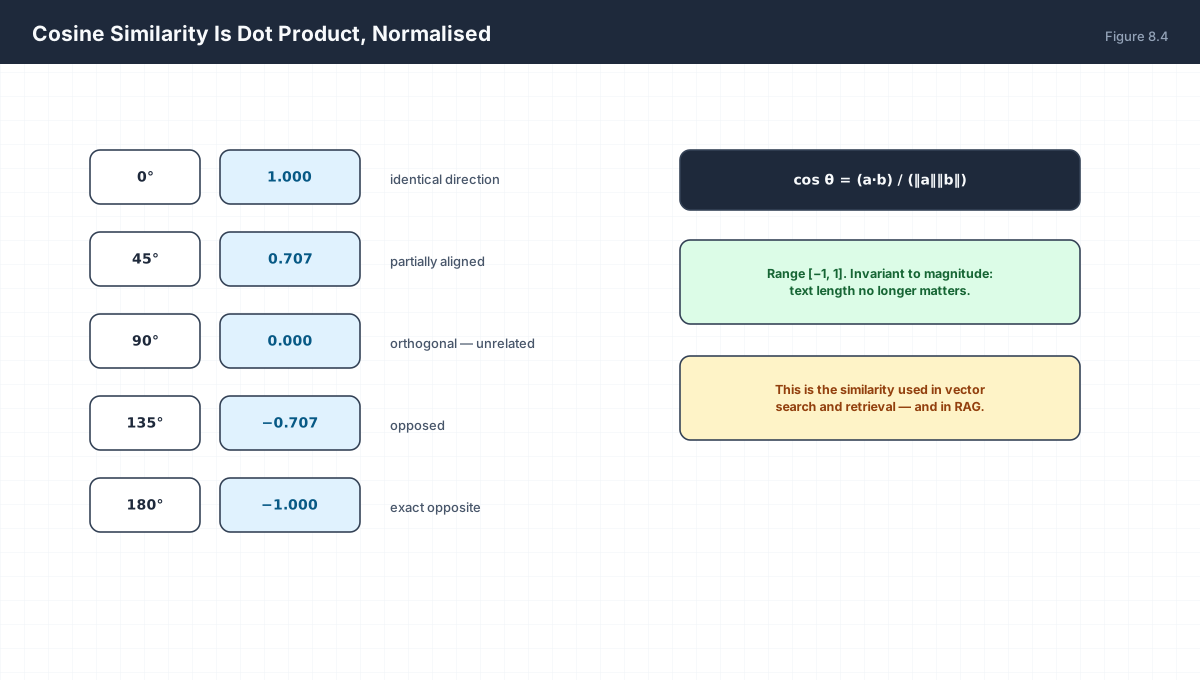
cos(u, v) = (u · v) / (‖u‖ ‖v‖)

Invariant to magnitude:  cos(2u, v) = cos(u, v)
This is why text retrieval normalises before comparing:
a long document and a short one about the same topic
should score 1.0, not "long beats short".
For unit vectors the cosine similarity and the dot product are identical, which is why retrieval pipelines normalise embeddings once at index time rather than dividing at query time.
6. One Operation, Three Disguises
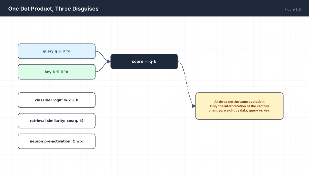
| Context | Expression | What the Vectors Are |
|---|---|---|
| Classifier | w·x + b |
weight vs input |
| Retrieval | cos(q, k) |
query vs document key |
| Attention | q·k / √d |
query vs key projections |
| Neuron | Σ wᵢxᵢ |
incoming weights vs activations |
6.1 Why attention divides by √d
If the components of q and k are independent with mean 0 and variance 1, their dot product over d dimensions has variance d and standard deviation √d. Changing d from 64 to 768 would make attention logits roughly 3.5× larger in magnitude, pushing softmax into saturation where gradients vanish. Dividing by √d restores unit variance, making the same temperature work at every width.
import numpy as np

rng = np.random.default_rng(0)
for d in (16, 64, 256, 1024):
    q = rng.normal(size=(2000, d))
    k = rng.normal(size=(2000, d))
    dots = np.sum(q * k, axis=1)
    print(f"d={d:5d}  std(dot)={dots.std():7.3f}  std(dot/√d)={ (dots/np.sqrt(d)).std():.3f}")
The second column grows like √d; the third is stable at 1.0. That stability is the entire justification for the scaling factor.
7. Worked Examples
7.1 Add, scale, and normalise
u = (1, 2),  v = (3, -1)
u + v      = (4, 1)
2u − 3v    = (2−9, 4+3) = (−7, 7)
‖2u − 3v‖  = √(49+49) = 9.899
7.2 Angle between two vectors
a = (1, 0),  b = (1, 1)
a·b = 1       ‖a‖ = 1, ‖b‖ = √2
cos θ = 1/√2 = 0.7071   →   θ = 45°
7.3 Norm comparison on the same vector
x = (3, -4)
L1 = 7, L2 = 5, L∞ = 4
Always:  L∞ ≤ L2 ≤ L1   for the same vector
7.4 Projection with a residual check
project b = (2,3) onto a = (4,0)
a·b = 8,  a·a = 16,  t = 0.5
proj = (2, 0)
residual = (0, 3),  and (0,3)·(4,0) = 0   ✓ orthogonal
7.5 Gradient clipping by norm
g = (30, 40),  ‖g‖ = 50,  clip = 1.0
g_clipped = g · (1/50) = (0.6, 0.8)     ‖g_clipped‖ = 1.0
Direction preserved, magnitude bounded.
8. Verify It in Python
import numpy as np

# --- 1. arithmetic identities --------------------------------------
u, v = np.array([1., 2.]), np.array([3., -1.])
assert np.allclose(u + v, [4., 1.])
assert np.allclose(2 * u - 3 * v, [-7., 7.])
print("linear combos ok")

# --- 2. norm ordering ----------------------------------------------
x = np.array([3., -4.])
n1, n2, ni = np.linalg.norm(x, 1), np.linalg.norm(x, 2), np.linalg.norm(x, np.inf)
assert ni <= n2 <= n1
print("Linf <= L2 <= L1:", ni, n2, n1)

# --- 3. dot product as projection ----------------------------------
a, b = np.array([4., 0.]), np.array([2., 3.])
assert np.isclose(a @ b, 8.0)
proj = (a @ b) / (a @ a) * a
assert np.allclose(proj, [2., 0.])
assert np.isclose((b - proj) @ a, 0.0)          # residual orthogonal
print("projection:", proj)

# --- 4. cosine is scale invariant ----------------------------------
def cos(u, v):
    return (u @ v) / (np.linalg.norm(u) * np.linalg.norm(v))

assert np.isclose(cos(a, b), cos(a * 7.5, b * 0.3))
assert np.isclose(cos(np.array([1., 0.]), np.array([1., 1.])), 1 / np.sqrt(2))
print("cosine invariant to magnitude")

# --- 5. orthogonal vectors have zero dot ---------------------------
assert np.isclose(np.array([1., 0.]) @ np.array([0., 1.]), 0.0)
print("orthogonal dot is zero")

# --- 6. dot product std grows as sqrt(d) ---------------------------
rng = np.random.default_rng(0)
stds = {}
for d in (16, 256, 1024):
    q = rng.normal(size=(4000, d)); k = rng.normal(size=(4000, d))
    stds[d] = np.sum(q * k, axis=1).std()
assert stds[1024] > 3 * stds[16]                 # grows with dimension
assert np.isclose(stds[1024] / np.sqrt(1024), 1.0, atol=0.1)
print("std(dot) by d:", {k: round(v, 2) for k, v in stds.items()})

# --- 7. clipping preserves direction -------------------------------
g = np.array([30., 40.])
gc = g * (1.0 / np.linalg.norm(g))
assert np.isclose(np.linalg.norm(gc), 1.0)
assert np.isclose(cos(g, gc), 1.0)
print("clipped:", gc)
print("all assertions passed")
9. Practice Questions
- Compute
(2,3,−1) + (−1,0,4)and its L2 norm. - For
x = (1,2,2), compute L1, L2, and L∞. - Find the angle between
(1,0)and(1,√3). - Show that
u·v = 0implies‖u+v‖² = ‖u‖² + ‖v‖². - Compute the projection of
(3,4)onto(1,0), and the residual. - Why is cosine similarity preferred over dot product for text retrieval?
- Derive why
Var(q·k) = dwhen components are i.i.d. unit variance. - What does dividing attention logits by
√dprotect against? - Clip a gradient
(6,8)to norm 2.0 and verify the direction is unchanged. - Explain geometrically why the L1 ball’s corners produce sparse solutions.
10. Official References & Further Reading
Continue the Course
- Course Index: AI Mathematics Masterclass — All 48 Chapters
- Previous Chapter: Chapter 7: Scalars, Vectors & Vector Spaces
- Next Chapter: Chapter 9: Matrices & Matrix Operations
- Related Series: PyTorch Engineering Masterclass — All 16 Modules