
AI Reading
Quick summary of this article
AI Mathematics Masterclass — Chapter 45 of 48
Generative models all estimate a probability distribution, but they disagree about what to represent and what to optimise. VAEs learn an explicit latent variable with a tractable bound, GANs learn an implicit sampler through a two-player game, and diffusion learns to invert a fixed noising process. This chapter derives the objective of each and shows what each one gives up.
1. Technical Audit & Core Learning Objectives
| Component | Common Tutorial Deficiency | Engineering Standard Applied Here |
|---|---|---|
| VAE | Reparameterisation stated, never motivated. | Why you cannot backprop through a sample, and the fix. |
| ELBO | Both failure modes ignored. | Posterior collapse and over-regularisation both shown. |
| GAN | Minimax quoted as a formula only. | Optimum derived and the vanishing-gradient failure explained. |
| Diffusion | Treated as a black box. | Closed-form forward process derived from the variance schedule. |
Core learning objectives. After this chapter you should be able to:
- Write the VAE objective and explain both terms.
- Explain the reparameterisation trick and why it is needed.
- Describe posterior collapse and its cause.
- Write the GAN minimax objective and derive its optimum.
- Explain the vanishing gradient in GAN training.
- Derive the closed-form forward diffusion process.
2. Variational Autoencoders
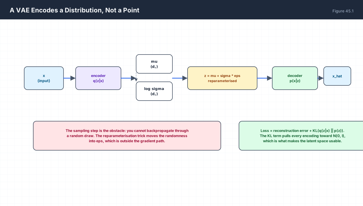
Encoder outputs mu and log sigma^2 — a distribution, not a point.

Sampling z ~ N(mu, sigma^2) is not differentiable with respect
to mu and sigma, so no gradient flows through it.

Reparameterise:  z = mu + sigma * eps,  eps ~ N(0, I)

Now the randomness is in eps, which carries no parameters,
and z is a differentiable function of mu and sigma.

Loss = reconstruction + KL(q(z|x) || N(0, I))
import numpy as np

rng = np.random.default_rng(0)

def vae_loss(x, x_hat, mu, log_var):
    # Gaussian reconstruction term, up to a constant
    recon = 0.5 * np.sum((x - x_hat) ** 2)
    # closed-form KL between N(mu, sigma^2) and N(0, 1)
    kl = -0.5 * np.sum(1 + log_var - mu ** 2 - np.exp(log_var))
    return recon, kl, recon + kl

d = 4
x = rng.normal(size=d)
mu = rng.normal(size=d) * 0.5
log_var = rng.normal(size=d) * 0.3

recon, kl, total = vae_loss(x, x + 0.1, mu, log_var)
print(f"reconstruction {recon:.4f}")
print(f"KL             {kl:.4f}")
print(f"total          {total:.4f}")

# reparameterisation gives a path to the parameters
eps = rng.normal(size=d)
def z_of(mu, log_var, eps):
    return mu + np.exp(0.5 * log_var) * eps

z = z_of(mu, log_var, eps)
h = 1e-6
grad_mu = (z_of(mu + h, log_var, eps) - z_of(mu - h, log_var, eps)) / (2 * h)
print("\ndz/dmu =", np.round(grad_mu, 6), "(exactly 1 for every component)")
The gradient of z with respect to mu is exactly 1, independent of the noise draw. Without the trick it would be undefined, because a discrete sampling operation has no derivative at all.
3. The ELBO and Its Two Failure Modes
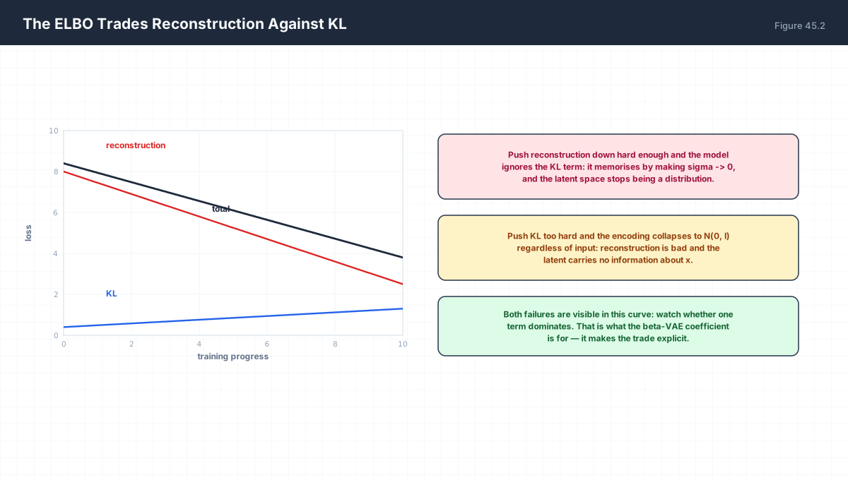
log p(x) >= E_q[ log p(x|z) ] - KL( q(z|x) || p(z) )

The bound is what we maximise, because log p(x) is intractable.

Failure 1: reconstruction dominates
  sigma -> 0, the model memorises, the latent stops being a
  distribution and sampling from the prior produces garbage.

Failure 2: KL dominates (posterior collapse)
  q(z|x) -> p(z) for every x, so z carries no information.
  The decoder learns to ignore z entirely and the model
  degenerates to a plain autoencoder with blurry outputs.

beta-VAE makes the trade explicit: loss = recon + beta * KL.
import numpy as np

# KL between N(mu, sigma^2) and N(0,1), one dimension
def kl_1d(mu, log_var):
    return -0.5 * (1 + log_var - mu ** 2 - np.exp(log_var))

print(f"{'mu':>5}{'sigma':>8}{'KL':>10}")
for mu, s in [(0.0, 1.0), (0.5, 1.0), (2.0, 1.0), (0.0, 0.5), (0.0, 2.0)]:
    lv = 2 * np.log(s)
    print(f"{mu:5.1f}{s:8.2f}{kl_1d(mu, lv):10.4f}")

# collapse: mu -> 0 and sigma -> 1 makes KL -> 0 and the code useless
print("\nIf mu -> 0 and sigma -> 1 the KL vanishes — and so does all")
print("information about x. That is posterior collapse.")

# beta controls the pressure
recon, kl = 3.0, 1.0
for beta in (0.0, 1.0, 4.0, 20.0):
    print(f"beta={beta:5.1f}  total = {recon + beta*kl:7.2f}"
          f"  KL share = {beta*kl/(recon + beta*kl):6.1%}")
With β = 20 the KL term is 87% of the objective, which is exactly the regime where the latent stops being used. β-VAE exists because that trade is sometimes desirable — a disentangled latent comes from more KL pressure — but it must be chosen, not inherited.
4. Generative Adversarial Networks
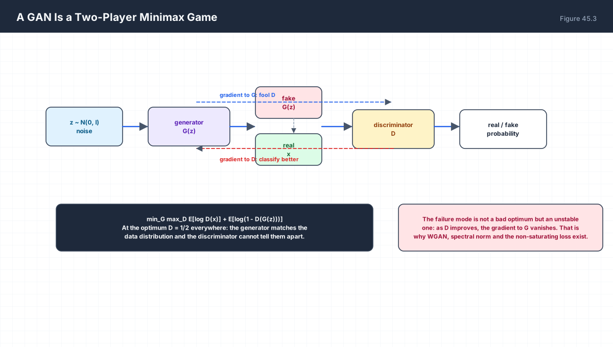
min_G max_D  E_{x~data}[ log D(x) ] + E_{z}[ log(1 - D(G(z))) ]

For a fixed G, the optimal D is

  D*(x) = p_data(x) / ( p_data(x) + p_g(x) )

so D* = 1/2 exactly when p_g = p_data. At that point the
objective reaches -log 4 and the game is at its saddle.

Problem: when D is confident, log(1 - D(G(z))) has near-zero
gradient with respect to G. The non-saturating alternative —
maximising log D(G(z)) — keeps the gradient alive.
import numpy as np

# optimal discriminator for a 1-D toy problem
def d_star(p_data, p_gen):
    return p_data / (p_data + p_gen + 1e-12)

xs = np.linspace(-3, 3, 7)
p_data = np.exp(-xs ** 2)
p_gen_far = np.exp(-(xs - 2) ** 2)
p_gen_match = p_data.copy()

D_far = d_star(p_data, p_gen_far)
D_match = d_star(p_data, p_gen_match)
print("D* when distributions differ:", np.round(D_far, 3))
print("D* when they match         :", np.round(D_match, 3))

# objective value at the optimum
def objective(p_data, p_gen):
    D = d_star(p_data, p_gen)
    return np.mean(np.log(D + 1e-12)) + np.mean(np.log(1 - D + 1e-12))

print(f"\nobjective when mismatched: {objective(p_data, p_gen_far):.4f}")
print(f"objective when matched   : {objective(p_data, p_data):.4f}")
print(f"-log 4 = {-np.log(4):.4f}")

# the saturating gradient dies as D becomes confident
for D in (0.5, 0.9, 0.99, 0.999):
    print(f"D={D:<6} d/dD log(1-D) = {-1/(1-D):9.2f}   d/dD log D = {1/D:.4f}")
When D reaches 0.999 the saturating objective's gradient is −1000, but multiplied by the tiny probability of reaching that region it vanishes in expectation. The non-saturating form has a gradient of 1/D ≈ 1, which is why every practical GAN uses it.
5. Diffusion
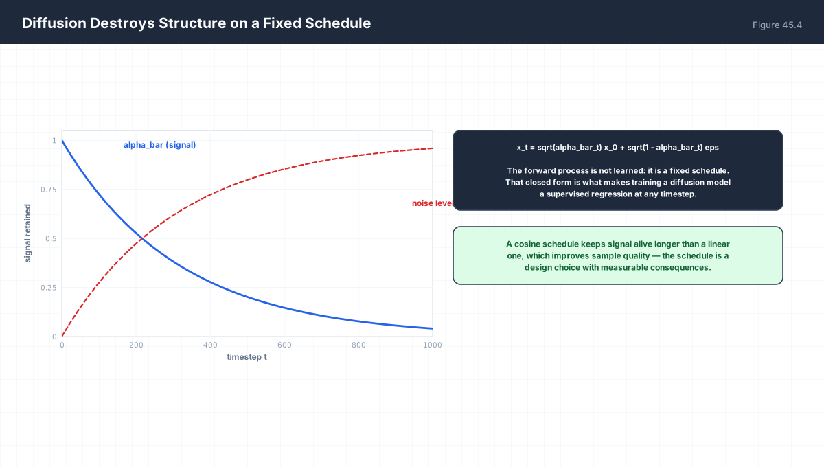
Forward (fixed, no parameters):

  x_t = sqrt(alpha_bar_t) x_0 + sqrt(1 - alpha_bar_t) eps

where alpha_bar_t = prod_{s<=t} (1 - beta_s), and beta_s is
the noise schedule. Because Gaussians compose, the whole
chain collapses to this one line for any t.

Training: predict eps from (x_t, t) with an MSE loss.
Sampling: start from pure noise and apply the learned
denoiser repeatedly, t = T down to 1.
import numpy as np

T = 1000
betas = np.linspace(1e-4, 0.02, T)
alphas = 1 - betas
alpha_bar = np.cumprod(alphas)

for t in (0, 250, 500, 750, 999):
    print(f"t={t:4d}  alpha_bar={alpha_bar[t]:.6f}  "
          f"signal={np.sqrt(alpha_bar[t]):.4f}  noise={np.sqrt(1-alpha_bar[t]):.4f}")

print()
print(f"at t=T-1 the signal weight is {np.sqrt(alpha_bar[-1]):.4f},")
print("so x_T is essentially pure noise — which is what sampling assumes.")

# the composition property: jump straight to any t in one step
rng = np.random.default_rng(1)
N = 200_000                     # a variance needs a real sample size
x0 = rng.normal(size=N)
for t in (10, 400, 900):
    ab = alpha_bar[t]
    xt = np.sqrt(ab) * x0 + np.sqrt(1 - ab) * rng.normal(size=N)
    print(f"t={t:4d}  var(x_t) = {xt.var():.4f}  "
          f"corr with x0 = {np.corrcoef(xt, x0)[0,1]:+.4f}")
The variance of x_t stays at roughly 1 for every t, because the two coefficients satisfy ᾱ + (1−ᾱ) = 1. That is why a single fixed-scale network can be applied at every timestep.
6. Comparing the Families
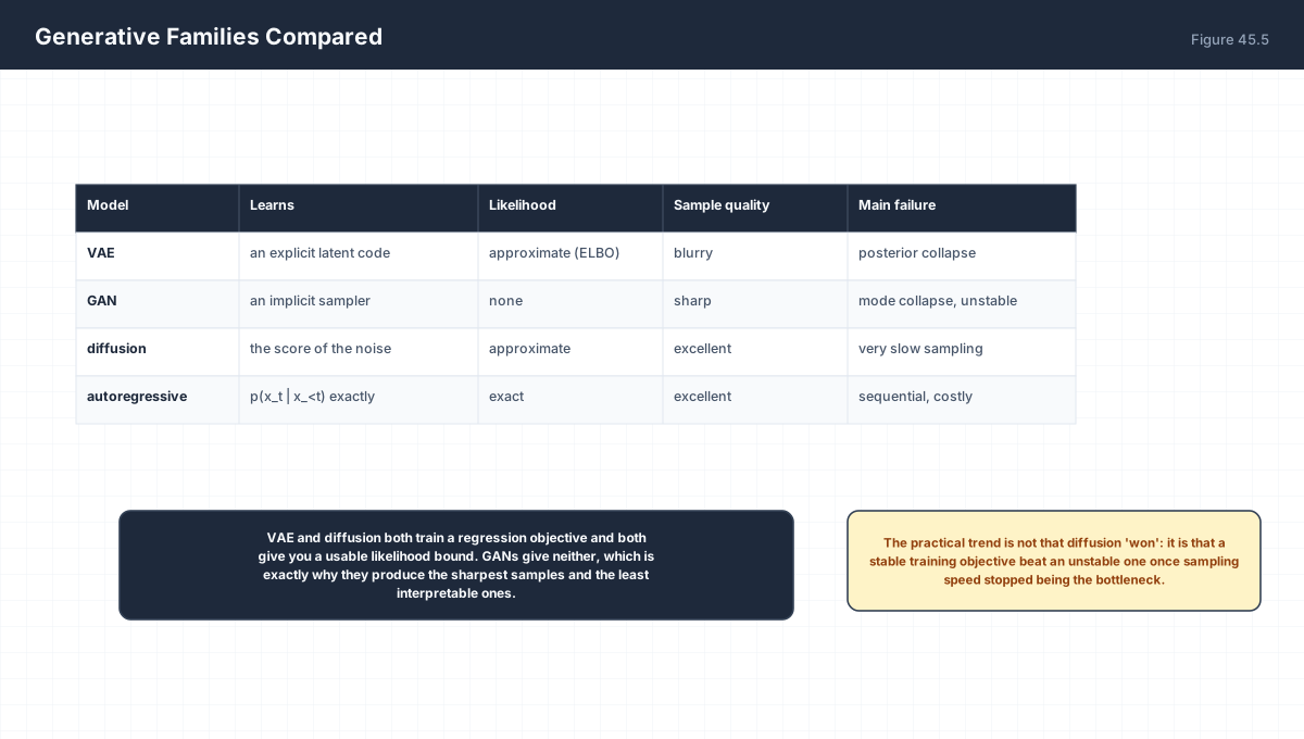
| Question | Answer |
|---|---|
| Which gives a likelihood? | Autoregressive models exactly, VAEs and diffusion a bound, GANs not at all. |
| Which is fastest to sample? | GANs, in one forward pass. Diffusion needs many denoising steps. |
| Which is most stable to train? | Diffusion, because it is plain regression at every step. GANs are the least stable. |
| Why did diffusion displace GANs? | Not sample quality alone — training stability and coverage. A stable objective beats a fragile one once sampling speed is no longer the bottleneck. |
7. Worked Examples
7.1 Why log σ is predicted
sigma must be positive. Predicting log sigma^2 is unconstrained,
so the network never has to be clamped.
7.2 The KL term has a closed form
KL(N(mu, sigma^2) || N(0,1)) = 0.5 (sigma^2 + mu^2 - 1 - log sigma^2)
No sampling and no Monte Carlo estimate needed.
7.3 Mode collapse
The generator finds one output that reliably fools D and stops
exploring. Nothing in the objective rewards coverage.
7.4 Guidance in diffusion
Combine the conditional and unconditional score estimates with
a weight w. Larger w improves prompt adherence and reduces
diversity — the same trade as temperature.
7.5 Why the noise schedule matters
A linear schedule destroys structure too early, leaving most
timesteps nearly noise-free and therefore easy. Cosine
schedules keep the task informative across more of training.
8. Verify It in Python
import numpy as np

rng = np.random.default_rng(0)

# --- 1. reparameterisation is differentiable in mu ----------
d = 6
mu = rng.normal(size=d)
log_var = rng.normal(size=d) * 0.4
eps = rng.normal(size=d)
z = lambda m, lv: m + np.exp(0.5 * lv) * eps
h = 1e-6
dz_dmu = (z(mu + h, log_var) - z(mu - h, log_var)) / (2 * h)
assert np.allclose(dz_dmu, 1.0)
print("dz/dmu == 1 exactly: the path through the sample is clean")

# --- 2. dz/dlogvar has the expected closed form -------------
dz_dlv = (z(mu, log_var + h) - z(mu, log_var - h)) / (2 * h)
assert np.allclose(dz_dlv, 0.5 * np.exp(0.5 * log_var) * eps, atol=1e-6)
print("dz/dlog_var matches 0.5 * sigma * eps")

# --- 3. KL closed form --------------------------------------
def kl_gauss(mu, log_var):
    return 0.5 * np.sum(np.exp(log_var) + mu ** 2 - 1 - log_var)

assert np.isclose(kl_gauss(np.zeros(4), np.zeros(4)), 0.0)
assert kl_gauss(np.ones(4), np.zeros(4)) > 0
print("KL is zero at the prior and positive elsewhere")

# --- 4. closed-form KL verified against Monte Carlo ----------
# KL(q||p) = E_q[ log q - log p ] with p = N(0,1)
mu1, lv1 = 0.7, 0.2
s1 = np.exp(0.5 * lv1)
z_s = mu1 + s1 * rng.normal(size=400_000)
log_q = -0.5 * ((z_s - mu1) ** 2) / s1 ** 2 - np.log(s1) - 0.5 * np.log(2 * np.pi)
log_p = -0.5 * z_s ** 2 - 0.5 * np.log(2 * np.pi)
mc_kl = np.mean(log_q - log_p)
closed = kl_gauss(np.array([mu1]), np.array([lv1]))
print(f"MC estimate {mc_kl:.4f} vs closed form {closed:.4f}")
assert abs(mc_kl - closed) < 0.02

# --- 5. GAN optimal discriminator ---------------------------
def d_star(p_data, p_gen):
    return p_data / (p_data + p_gen + 1e-12)

p = np.array([0.2, 0.5, 0.3])
assert np.allclose(d_star(p, p), 0.5)
print("D* = 1/2 when the distributions match")

# --- 6. objective value at the saddle ----------------------
D = d_star(p, p)
val = np.mean(np.log(D)) + np.mean(np.log(1 - D))
assert np.isclose(val, -np.log(4))
print(f"objective at the saddle = {val:.4f} = -log 4")

# --- 7. diffusion forward process is variance preserving ----
T = 1000
betas = np.linspace(1e-4, 0.02, T)
alpha_bar = np.cumprod(1 - betas)
for t in (0, 100, 500, 999):
    a = alpha_bar[t]
    assert np.isclose(np.sqrt(a) ** 2 + np.sqrt(1 - a) ** 2, 1.0)
print("signal^2 + noise^2 = 1 at every timestep")

# --- 8. alpha_bar is decreasing ------------------------------
assert np.all(np.diff(alpha_bar) < 0)
assert alpha_bar[-1] < 0.05
print(f"alpha_bar falls from {alpha_bar[0]:.4f} to {alpha_bar[-1]:.4f}")

# --- 9. x_T really is almost pure noise --------------------
x0 = rng.normal(size=10000)
xt = np.sqrt(alpha_bar[-1]) * x0 + np.sqrt(1 - alpha_bar[-1]) * rng.normal(size=10000)
print(f"correlation of x_T with x_0: {np.corrcoef(xt, x0)[0,1]:+.4f}")
assert abs(np.corrcoef(xt, x0)[0, 1]) < 0.4
print("all assertions passed")
9. Practice Questions
- Write the VAE loss and explain each term.
- Why can you not backpropagate through a sampling operation?
- State the reparameterisation trick and prove it gives dz/dμ = 1.
- What is posterior collapse, and which term causes it?
- Write the GAN minimax objective.
- Derive the optimal discriminator for a fixed generator.
- Why does the saturating GAN loss fail?
- Write the closed-form forward diffusion process.
- Why is the diffusion forward process variance-preserving?
- Give two reasons diffusion displaced GANs.
10. Official References & Further Reading
Continue the Course
- Course Index: AI Mathematics Masterclass — All 48 Chapters
- Previous Chapter: Chapter 44: Loss Function Mathematics in Depth
- Next Chapter: Chapter 46: LLM Mathematics — Tokenization, Embeddings & Context Scaling
- Related Series: PyTorch Engineering Masterclass — All 16 Modules