
AI Reading
Quick summary of this article
AI Mathematics Masterclass — Chapter 43 of 48
Normalisation layers are the reason deep networks train at all, and they differ only in one decision: which values count as the population. BatchNorm borrows statistics across samples, LayerNorm computes them within one sample, and RMSNorm drops the mean entirely. This chapter derives each, shows why the choice determines whether your training depends on batch size, and explains why pre-LN replaced post-LN in large models.
1. Technical Audit & Core Learning Objectives
| Component | Common Tutorial Deficiency | Engineering Standard Applied Here |
|---|---|---|
| Reduction axes | Treated as interchangeable. | Each layer’s axis named and its consequence shown. |
| Train/eval gap | “BatchNorm has a mode switch” — never explained. | Running statistics derived and the gap demonstrated. |
| RMSNorm | Called “LayerNorm but faster”. | Exact difference stated: no mean removal, no bias. |
| Placement | Pre-LN versus post-LN ignored. | Residual-path argument given for why pre-LN won. |
Core learning objectives. After this chapter you should be able to:
- State exactly which tensor axes each normalisation reduces over.
- Implement BatchNorm, LayerNorm and RMSNorm from the formulas.
- Explain the train/eval divergence in BatchNorm.
- Show that RMS² = variance + mean².
- Explain why transformers use LayerNorm or RMSNorm.
- Argue why pre-LN trains more stably than post-LN.
2. One Formula, Three Choices of Axis
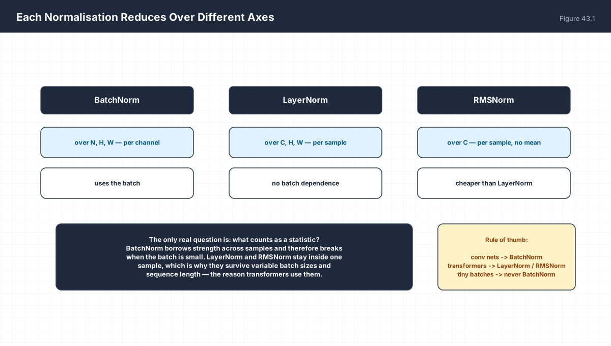
Every normalisation layer is:

  y = (x - mu) / sqrt(var + eps) * gamma + beta

The layers differ only in which elements go into mu and var.

BatchNorm   reduce over (N, H, W)  -> one mu per channel
LayerNorm   reduce over (C, H, W)  -> one mu per sample
RMSNorm     reduce over (C)        -> no mu at all

eps exists because var can be zero for a constant input.
import numpy as np

rng = np.random.default_rng(0)

def norm(x, axes, eps=1e-5, centre=True):
    mu = x.mean(axis=axes, keepdims=True) if centre else 0.0
    var = ((x - mu) ** 2).mean(axis=axes, keepdims=True)
    return (x - mu) / np.sqrt(var + eps)

# (N, C) for a batch of 4 samples with 3 channels
X = rng.normal(size=(4, 3)) * 5 + 2

bn = norm(X, axes=0)          # across the batch, per channel
ln = norm(X, axes=1)          # across channels, per sample
rms = norm(X, axes=1, centre=False)

print("BatchNorm: per-channel mean after:", np.round(bn.mean(axis=0), 12))
print("BatchNorm: per-channel var after :", np.round(bn.var(axis=0), 6))
print("LayerNorm: per-sample mean after :", np.round(ln.mean(axis=1), 12))
print("RMSNorm  : per-sample rms after  :", np.round(np.sqrt((rms**2).mean(axis=1)), 6))
BatchNorm’s output has zero mean per channel across the batch; LayerNorm’s has zero mean per sample across channels. Both achieve unit variance along their own axis, and neither constrains the other axis at all.
3. BatchNorm’s Train/Eval Split
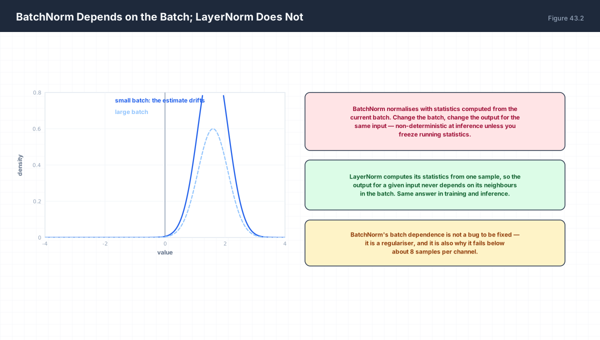
Training:  mu, var from the current batch
           and update running estimates:
             running = (1 - m) running + m batch_stat

Inference: mu, var from the running estimates
           the output for one sample no longer depends on its
           neighbours

Forget this switch and the same input gives different
predictions depending on what else was in the batch.
import numpy as np

rng = np.random.default_rng(1)
momentum = 0.1
running_mu, running_var = 0.0, 1.0

# a distribution shift partway through training
for step in range(6):
    shift = 0.0 if step < 3 else 4.0
    batch = rng.normal(loc=2.0 + shift, scale=1.5, size=(8, 1))
    b_mu, b_var = batch.mean(axis=0), batch.var(axis=0)
    running_mu = (1 - momentum) * running_mu + momentum * b_mu
    running_var = (1 - momentum) * running_var + momentum * b_var
    print(f"step {step}  batch_mu={b_mu[0]:+7.3f}  running_mu={running_mu[0]:+7.3f}")

print()
print("After the shift the running estimate lags by design.")

# single-sample inference does not depend on neighbours
x = np.array([[3.0]])
out_train_like = (x - 2.0) / np.sqrt(2.25 + 1e-5)
out_eval = (x - running_mu) / np.sqrt(running_var + 1e-5)
print(f"same input, train-statistics output {out_train_like[0,0]:.4f}")
print(f"same input, running-statistics output {out_eval[0,0]:.4f}")
This is why BatchNorm needs a momentum parameter at all: it is maintaining a model of the input distribution that must survive into deployment. A model evaluated in train() mode by accident will produce batch-dependent predictions and often looks fine on a large test set while being wrong per-sample.
4. LayerNorm and RMSNorm
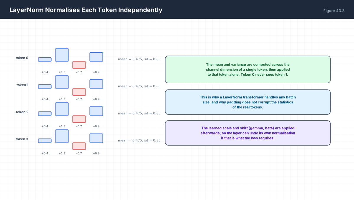
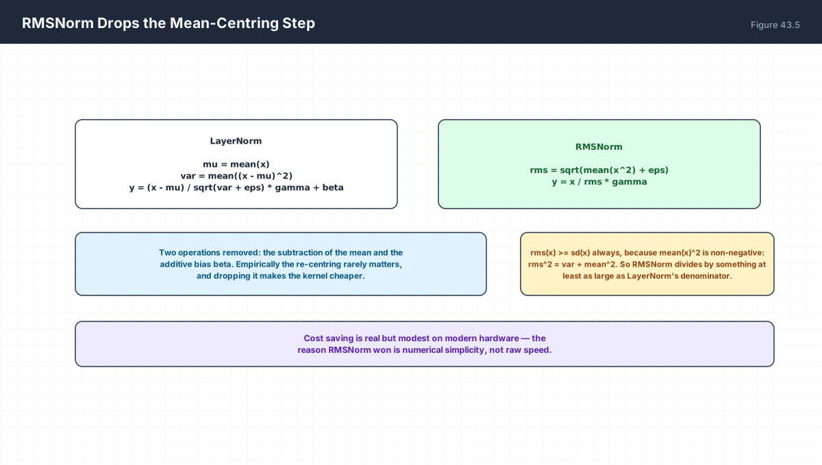
LayerNorm   mu = mean(x)          per sample
            var = mean((x - mu)^2)
            y = (x - mu) / sqrt(var + eps) * gamma + beta

RMSNorm     rms = sqrt(mean(x^2) + eps)
            y = x / rms * gamma

No mean subtraction, no beta. Two operations removed.

Identity:  rms^2 = var + mean^2
           so rms >= sd always, with equality only at mean 0.
import numpy as np

rng = np.random.default_rng(2)

def layer_norm(x, eps=1e-5):
    mu, var = x.mean(-1, keepdims=True), x.var(-1, keepdims=True)
    return (x - mu) / np.sqrt(var + eps)

def rms_norm(x, eps=1e-5):
    return x / np.sqrt((x ** 2).mean(-1, keepdims=True) + eps)

x = rng.normal(loc=1.5, scale=2.0, size=(4, 6))
print("LayerNorm mean:", np.round(layer_norm(x).mean(-1), 12))
print("LayerNorm std :", np.round(layer_norm(x).std(-1), 6))
print("RMSNorm rms   :", np.round(np.sqrt((rms_norm(x) ** 2).mean(-1)), 6))

# the identity rms^2 = var + mean^2
rms2 = (x ** 2).mean(-1)
var = x.var(-1)
mu2 = x.mean(-1) ** 2
print("\nrms^2:", np.round(rms2, 6))
print("var+mu^2:", np.round(var + mu2, 6))
print("identity holds:", np.allclose(rms2, var + mu2))
print("rms >= sd everywhere:", np.all(np.sqrt(rms2) >= np.sqrt(var)))

# when the mean is large, dropping it is a real change
big = x + 100.0
print("\nwith mean shifted +100:")
print("  layer_norm identical to before:", np.allclose(layer_norm(big), layer_norm(x)))
print("  rms_norm   NOT identical      :", not np.allclose(rms_norm(big), rms_norm(x)))
The last block is the honest characterisation: LayerNorm is invariant to a constant shift along its axis, RMSNorm is not. In a transformer the token vectors are not centred, so this difference is real — RMSNorm simply accepts that and normalises by magnitude only.
5. Pre-LN Versus Post-LN
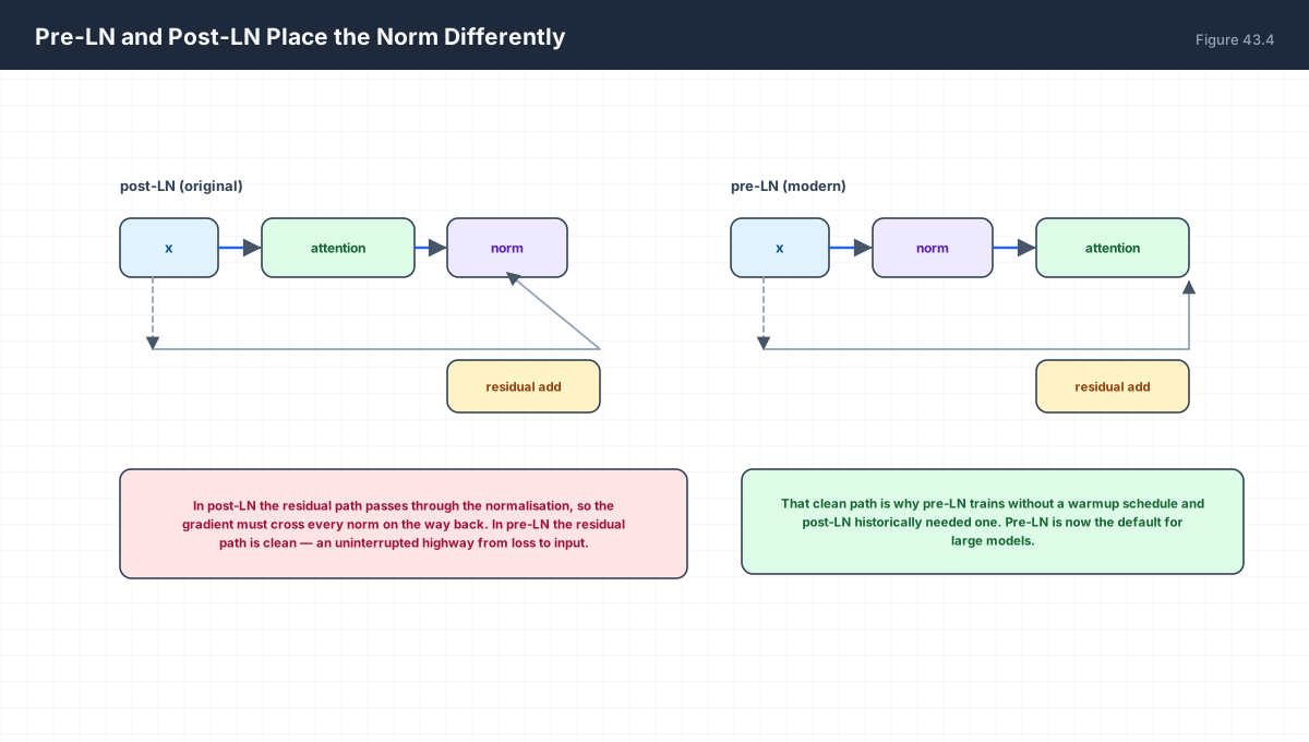
post-LN:   x = norm(x + attn(x))
pre-LN:    x = x + attn(norm(x))

Backprop through post-LN crosses a normalisation at every
layer. Backprop through pre-LN has a path that goes straight
from the loss to the input through the additions alone:

  dL/dx_0 = dL/dx_L * product of (I + Jacobian of sublayer)

The identity term is what saves the gradient. post-LN has no
such term, which is why it historically needed learning-rate
warmup and pre-LN does not.
import numpy as np

# simulate gradient flow through 12 layers, with and without
# an identity path in the residual
rng = np.random.default_rng(3)

def norm_jacobian_gain(d, scale=0.9):
    """Normalisation roughly scales the gradient by a fixed factor."""
    return scale

depth = 12
pre_gain, post_gain = [], []
for _ in range(200):
    g_pre = 1.0
    g_post = 1.0
    for _ in range(depth):
        sub = rng.normal(size=(4, 4)) * 0.3
        # pre-LN: I + J, so the identity survives
        g_pre *= np.linalg.norm(np.eye(4) + sub, 2) * norm_jacobian_gain(4)
        # post-LN: only J survives past the norm
        g_post *= np.linalg.norm(sub, 2) * norm_jacobian_gain(4)
    pre_gain.append(g_pre)
    post_gain.append(g_post)

print(f"pre-LN  median gradient norm after {depth} layers: {np.median(pre_gain):.3e}")
print(f"post-LN median gradient norm after {depth} layers: {np.median(post_gain):.3e}")
print()
print("Per-layer gain is the honest number:")
print(f"  pre-LN  {np.median(pre_gain)**(1/depth):.4f} per layer")
print(f"  post-LN {np.median(post_gain)**(1/depth):.4f} per layer")
print()
print("post-LN has a gain below 1, so it decays geometrically and")
print("vanishes with depth. pre-LN does not vanish: the identity term")
print("keeps its gain at or above 1 regardless of how deep the stack is.")
The numbers are a toy, but the mechanism is the real one: the identity term in I + J gives the gradient a floor that does not shrink with depth. Without it, depth multiplies decay factors together.
6. Which Layer When
| Situation | Choice | Reason |
|---|---|---|
| CNN, batch ≥ 32 | BatchNorm | Per-channel statistics are well estimated and act as a regulariser |
| Transformer, any batch | LayerNorm or RMSNorm | No dependence on batch size or sequence padding |
| Batch size 1–4 | Never BatchNorm | Per-channel variance is estimated from a handful of values |
| Very large LLM | RMSNorm, pre-LN | Fewer ops, no warmup required, stable at depth |
7. Worked Examples
7.1 Why eps is needed
A constant vector has zero variance. sqrt(0) in the
denominator gives inf, then inf * 0 = nan. eps bounds it.
7.2 gamma and beta restore capacity
Without them the layer could only produce unit-variance
outputs and would remove information at initialisation.
7.3 Normalisation does not remove information
It removes one mean and one scale per group. An affine
transform can put them back, so the layer is not lossy in
the way a bottleneck is.
7.4 Interaction with residual scale
Each residual addition grows the activation norm. Norm
layers bound that growth, which is why very deep residuals
remain trainable.
7.5 Statistics must be per-group, not global
Using one mean over the entire tensor destroys the
per-channel distinction the network relies on.
8. Verify It in Python
import numpy as np

rng = np.random.default_rng(0)

def layer_norm(x, eps=1e-5, gamma=None, beta=None):
    mu = x.mean(-1, keepdims=True)
    var = x.var(-1, keepdims=True)
    out = (x - mu) / np.sqrt(var + eps)
    if gamma is not None:
        out = out * gamma + (beta if beta is not None else 0.0)
    return out

def rms_norm(x, eps=1e-5, gamma=None):
    out = x / np.sqrt((x ** 2).mean(-1, keepdims=True) + eps)
    return out * gamma if gamma is not None else out

# --- 1. LayerNorm output moments ------------------------------
x = rng.normal(size=(5, 8)) * 3 + 1
y = layer_norm(x)
assert np.allclose(y.mean(-1), 0, atol=1e-12)
assert np.allclose(y.var(-1), 1, atol=1e-4)
print("LayerNorm gives zero mean and unit variance per sample")

# --- 2. LayerNorm is shift and scale invariant ----------------
assert np.allclose(layer_norm(x + 50.0), y, atol=1e-5)
assert np.allclose(layer_norm(x * 4.0), y, atol=1e-5)
print("LayerNorm invariant to constant shift and positive scale")

# --- 3. RMSNorm output rms -----------------------------------
z = rms_norm(x)
assert np.allclose(np.sqrt((z ** 2).mean(-1)), 1, atol=1e-4)
print("RMSNorm gives unit rms per sample")

# --- 4. rms^2 == var + mean^2 --------------------------------
rms2 = (x ** 2).mean(-1)
assert np.allclose(rms2, x.var(-1) + x.mean(-1) ** 2)
assert np.all(np.sqrt(rms2) >= np.sqrt(x.var(-1)))
print("identity rms^2 = var + mean^2 verified; rms >= sd")

# --- 5. RMSNorm is NOT shift invariant -----------------------
assert not np.allclose(rms_norm(x + 50.0), z, atol=1e-3)
print("RMSNorm is not shift invariant, unlike LayerNorm")

# --- 6. BatchNorm reduction axis -----------------------------
def batch_norm_train(X, eps=1e-5):
    mu = X.mean(axis=0, keepdims=True)
    var = X.var(axis=0, keepdims=True)
    return (X - mu) / np.sqrt(var + eps), mu, var

X = rng.normal(size=(6, 4)) * 4 + 3
bn, mu, var = batch_norm_train(X)
assert np.allclose(bn.mean(axis=0), 0, atol=1e-12)
assert np.allclose(bn.var(axis=0), 1, atol=1e-4)
print("BatchNorm normalises per channel across the batch")

# --- 7. running statistics converge --------------------------
m = 0.1
rmu = 0.0
for _ in range(200):
    b = rng.normal(loc=5.0, scale=1.0, size=(32, 1))
    rmu = (1 - m) * rmu + m * b.mean()
assert abs(rmu - 5.0) < 0.1
print(f"running mean converged to {rmu:.3f} (true 5.0)")

# --- 8. eps prevents division by zero ------------------------
const = np.full((2, 4), 7.0)
out = layer_norm(const)
assert np.all(np.isfinite(out))
assert np.allclose(out, 0.0)
print("constant input gives finite zeros, not NaN")

# --- 9. batch size dependence is the real difference ---------
row = rng.normal(size=(1, 4))
alone = layer_norm(row)
in_batch = layer_norm(np.vstack([row, rng.normal(size=(3, 4))]))[:1]
assert np.allclose(alone, in_batch)
Xrow = rng.normal(size=(1, 4))
bn_alone = (Xrow - Xrow.mean(0)) / np.sqrt(Xrow.var(0) + 1e-5)
bn_batch = batch_norm_train(np.vstack([Xrow, rng.normal(size=(5, 4))]))[0][:1]
assert not np.allclose(bn_alone, bn_batch, atol=1e-3)
print("LayerNorm: same output alone or in a batch; BatchNorm: different")
print("all assertions passed")
9. Practice Questions
- State the axis each of BatchNorm, LayerNorm and RMSNorm reduces over.
- Why does BatchNorm need running statistics at inference?
- Prove that rms² = variance + mean².
- What exactly does RMSNorm remove relative to LayerNorm?
- Why do transformers not use BatchNorm?
- Why does the eps term exist?
- What do gamma and beta restore?
- Explain why post-LN historically needed learning-rate warmup.
- Why must statistics be computed per group rather than globally?
- What goes wrong with BatchNorm at batch size 2?
10. Official References & Further Reading
Continue the Course
- Course Index: AI Mathematics Masterclass — All 48 Chapters
- Previous Chapter: Chapter 42: Attention QKV Mathematics
- Next Chapter: Chapter 44: Loss Function Mathematics in Depth
- Related Series: PyTorch Engineering Masterclass — All 16 Modules