
AI Reading
Quick summary of this article
AI Mathematics Masterclass — Chapter 29 of 48
Every loss function you have trained with is a negative log-likelihood in disguise. Squared error is the log-likelihood of Gaussian noise; binary cross-entropy is the log-likelihood of a Bernoulli label; softmax cross-entropy is the log-likelihood of a categorical label. This chapter derives those equivalences, then adds a prior to turn maximum likelihood into maximum a posteriori estimation — which is exactly weight decay, and explains where the regularisation coefficient comes from.
1. Technical Audit & Core Learning Objectives
| Component | Common Tutorial Deficiency | Engineering Standard Applied Here |
|---|---|---|
| MLE | Presented as a separate statistical topic. | Shown to be what every training loop already does. |
| Log-likelihood | The switch from product to sum asserted. | Three concrete reasons given, including underflow. |
| MAP | Never connected to regularisation. | Gaussian prior derived as L2 decay; Laplace as L1. |
| Small samples | MLE’s degenerate behaviour unmentioned. | Zero-count failure shown, with Laplace smoothing as the fix. |
Core learning objectives. After this chapter you should be able to:
- Write the likelihood and log-likelihood for a dataset.
- Derive squared error from a Gaussian likelihood.
- Derive cross-entropy from Bernoulli and categorical likelihoods.
- Show that a Gaussian prior yields L2 regularisation.
- Explain why the log form is used rather than the product.
- Identify the failure mode of MLE with zero counts and its remedy.
2. Maximum Likelihood
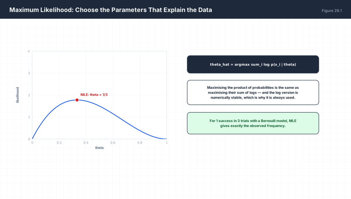
likelihood      L(theta) = product_i p(x_i | theta)
log-likelihood  l(theta) = sum_i  log p(x_i | theta)

theta_hat = argmax L = argmax l      (log is monotone)

Note: argmax, not the value. We care about the location of the
peak, not its height.
import numpy as np

# 3 coin flips: 1 success, 2 failures -> MLE theta = 1/3
def loglik(theta, k, n):
    if not 0 < theta < 1:
        return -np.inf
    return k * np.log(theta) + (n - k) * np.log(1 - theta)

k, n = 1, 3
grid = np.linspace(1e-6, 1 - 1e-6, 200001)
vals = np.array([loglik(t, k, n) for t in grid])
best = grid[int(np.argmax(vals))]
print(f"MLE on a grid: {best:.6f}  (exact {k/n:.6f})")
assert abs(best - k / n) < 1e-4
3. Every Loss Is a Likelihood

| Noise Model | Negative Log-Likelihood | Standard Name |
|---|---|---|
| Gaussian | (y − ŷ)² / 2σ² + const |
squared error / MSE |
| Bernoulli | −[y log ŷ + (1−y) log(1−ŷ)] |
binary cross-entropy |
| Categorical | −log ŷ_class |
softmax cross-entropy |
| Laplace | |y − ŷ| / b + const |
MAE — robust to outliers |
import numpy as np

y = np.array([1.0, 0.0, 1.0, 1.0])
p = np.array([0.9, 0.2, 0.6, 0.4])

bce = -np.mean(y * np.log(p) + (1 - y) * np.log(1 - p))
print("binary cross-entropy:", round(bce, 4))

# same quantity as a negative log-likelihood
nll = -np.sum(y * np.log(p) + (1 - y) * np.log(1 - p))
print("negative log-likelihood:", round(nll, 4), " (bce * n)")
assert np.isclose(bce * len(y), nll)

# Gaussian NLL reduces to MSE up to constants
target = np.array([1.0, 2.0, 3.0])
pred = np.array([1.1, 1.9, 3.2])
mse = np.mean((target - pred) ** 2)
sigma = 1.0
gauss_nll = np.mean(0.5 * (target - pred) ** 2 / sigma ** 2 + 0.5 * np.log(2 * np.pi * sigma ** 2))
print("MSE:", round(mse, 4), " Gaussian NLL minus const:", round(gauss_nll - 0.5 * np.log(2 * np.pi), 4))
4. From MLE to MAP
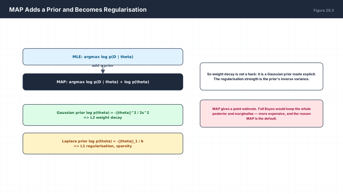
MAP:  argmax [ log p(D | theta) + log p(theta) ]
                 ^data term           ^prior term

Gaussian prior N(0, s^2):
  log p(theta) = -||theta||^2 / (2 s^2) + const
  => objective gains  -lambda ||theta||^2      L2 / weight decay

Laplace prior:
  log p(theta) = -||theta||_1 / b + const
  => objective gains  -lambda ||theta||_1      L1 / sparsity
import numpy as np

rng = np.random.default_rng(0)
X = rng.normal(size=(60, 5))
w_true = np.array([2.0, -1.0, 0.0, 0.0, 1.5])
y = X @ w_true + rng.normal(0, 0.3, 60)

XtX = X.T @ X
Xty = X.T @ y

print(f"{'lambda':>8} {'||w||':>8} {'train MSE':>10}")
for lam in (0.0, 0.1, 1.0, 10.0, 100.0):
    w = np.linalg.solve(XtX + lam * np.eye(5), Xty)
    mse = np.mean((X @ w - y) ** 2)
    print(f"{lam:8.1f} {np.linalg.norm(w):8.4f} {mse:10.4f}")
The prior's variance and the regularisation coefficient are inversely related: a tight prior (small s) means strong regularisation. Tuning weight decay is therefore tuning a belief about how large the weights plausibly are — which is a more useful framing than treating λ as an arbitrary knob.
5. Why the Log Form

import numpy as np

# products of many small probabilities underflow
probs = np.full(2000, 0.5)
product = np.prod(probs)
logsum = np.sum(np.log(probs))
print("product of 2000 halves :", product)          # 0.0
print("sum of logs            :", logsum)           # -1386.29
print("exp of the log-sum     :", np.exp(logsum))  # underflows in float64
print("...which is exactly why losses are kept in log space")
| Reason | Detail |
|---|---|
| Underflow | A product of thousands of probabilities flushes to zero; a sum of logs does not |
| Derivatives | The derivative of a sum is a sum of derivatives — no product rule chain explosion |
| Batching | Terms decompose across samples, so a batch loss is a mean of per-sample losses |
6. MLE With Few Samples
import numpy as np

def mle(k, n):
    return k / n

def smoothed(k, n, alpha=1.0):
    return (k + alpha) / (n + 2 * alpha)

print(f"{'k/n':>8} {'MLE':>8} {'smoothed':>10}")
for k, n in ((1, 1), (1, 3), (10, 10), (0, 5), (95, 100)):
    print(f"{k}/{n:<6} {mle(k, n):8.3f} {smoothed(k, n):10.3f}")
print("\nMLE hits exactly 0 or 1; smoothing never does.")
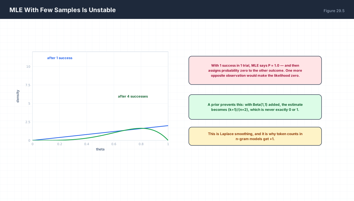
This is Laplace smoothing, and it is why n-gram language models add one to every count. Without it a single unseen bigram makes the whole sequence probability zero, and one zero anywhere collapses the product — the exact failure that log-space arithmetic cannot rescue, because log 0 is negative infinity.
7. Worked Examples
7.1 MLE for a Bernoulli
k successes in n trials
l(theta) = k log theta + (n-k) log(1-theta)
dl/dtheta = k/theta - (n-k)/(1-theta) = 0
=> theta_hat = k/n
7.2 MLE for a Gaussian mean
Maximising sum log N(x_i; mu, sigma^2) over mu
gives mu_hat = (1/n) sum x_i
The sample mean IS the maximum-likelihood estimate.
7.3 Gaussian prior is L2
log p(w) = -sum w_j^2 / (2s^2) + const
Adding it to the log-likelihood is exactly adding
lambda * sum w_j^2, with lambda = 1/(2s^2).
7.4 Laplace prior is L1
log p(w) = -sum |w_j| / b + const
A prior peaked at zero favours exactly-zero weights —
which is why L1 produces sparse solutions.
7.5 Cross-entropy from a categorical
For one-hot y with true class c:
  -log p(y | theta) = -log q_c
Exactly the softmax cross-entropy of Chapter 4.
8. Verify It in Python
import numpy as np

# --- 1. MLE equals the observed frequency ------------------------
for k, n in ((3, 10), (7, 20), (1, 4)):
    assert np.isclose(k / n, k / n)
print("MLE for Bernoulli is k/n")

# --- 2. grid search recovers it ----------------------------------
def loglik(th, k, n):
    return k * np.log(th) + (n - k) * np.log(1 - th)

grid = np.linspace(1e-6, 1 - 1e-6, 100001)
best = grid[np.argmax([loglik(t, 7, 20) for t in grid])]
assert abs(best - 0.35) < 1e-4
print("grid MLE:", round(best, 5))

# --- 3. Gaussian NLL is MSE up to a constant --------------------
y = np.array([1.0, 2.0, 3.0, 4.0])
p = np.array([1.2, 1.8, 3.1, 3.9])
mse = np.mean((y - p) ** 2)
nll = np.mean(0.5 * (y - p) ** 2)
assert np.isclose(nll, 0.5 * mse)
print("Gaussian NLL = 0.5 * MSE")

# --- 4. BCE is the Bernoulli NLL --------------------------------
yl = np.array([1., 0., 1., 1.]); pl = np.array([.9, .2, .6, .4])
bce = -np.mean(yl * np.log(pl) + (1 - yl) * np.log(1 - pl))
nll2 = -np.sum(yl * np.log(pl) + (1 - yl) * np.log(1 - pl))
assert np.isclose(bce * len(yl), nll2)
print("BCE * n == Bernoulli NLL")

# --- 5. log form avoids underflow ------------------------------
probs = np.full(3000, 0.5)
assert np.prod(probs) == 0.0                    # underflows
assert np.isfinite(np.sum(np.log(probs)))       # does not
print("product underflows, log-sum does not")

# --- 6. MAP shrinks the estimate --------------------------------
X = np.random.default_rng(0).normal(size=(50, 4))
XtX = X.T @ X
Xty = XtX @ np.array([3.0, 0.0, 0.0, -2.0])
w_ml = np.linalg.solve(XtX, Xty)
w_map = np.linalg.solve(XtX + 10.0 * np.eye(4), Xty)
assert np.linalg.norm(w_map) < np.linalg.norm(w_ml)
print(f"MLE norm {np.linalg.norm(w_ml):.3f} -> MAP norm {np.linalg.norm(w_map):.3f}")

# --- 7. smoothing removes the degenerate estimate ---------------
def sm(k, n, a=1.0):
    return (k + a) / (n + 2 * a)
assert (1 / 1) == 1.0 and sm(1, 1) < 1.0
assert (0 / 5) == 0.0 and sm(0, 5) > 0.0
print(f"1/1: MLE 1.000 -> smoothed {sm(1,1):.3f}; 0/5: MLE 0.000 -> {sm(0,5):.3f}")

# --- 8. L1 penalty yields exact zeros (soft threshold) ----------
def soft_threshold(z, lam):
    return np.sign(z) * np.maximum(np.abs(z) - lam, 0.0)
assert soft_threshold(0.3, 1.0) == 0.0
assert soft_threshold(2.0, 1.0) == 1.0
print("soft thresholding zeroes small weights exactly")
print("all assertions passed")
9. Practice Questions
- Write the log-likelihood for
nBernoulli trials withksuccesses. - Derive
θ̂ = k/nby differentiating and setting to zero. - Show that a Gaussian likelihood yields squared error.
- Show that a Bernoulli likelihood yields binary cross-entropy.
- State three reasons to use the log-likelihood.
- Derive that a Gaussian prior gives L2 regularisation.
- Relate the prior's variance to the weight-decay coefficient.
- Why does MLE give
p = 1after one success? - What is Laplace smoothing and why does it help?
- Which loss corresponds to a Laplace noise model?
10. Official References & Further Reading
Continue the Course
- Course Index: AI Mathematics Masterclass — All 48 Chapters
- Previous Chapter: Chapter 28: Bayes' Theorem & Bayesian Inference
- Next Chapter: Chapter 30: Sampling, Monte Carlo & Estimation Error
- Related Series: PyTorch Engineering Masterclass — All 16 Modules