
AI Reading
Quick summary of this article
AI Mathematics Masterclass — Chapter 32 of 48
Hypothesis testing is the machinery for deciding whether an observed difference is real or noise. Its logic is indirect — you assume no effect and ask how surprising the data would be — and that indirection is the source of nearly every misuse. This chapter covers the null hypothesis, the two error types, the two-sided rejection region, and why a confidence interval communicates more than a p-value.
1. Technical Audit & Core Learning Objectives
| Component | Common Tutorial Deficiency | Engineering Standard Applied Here |
|---|---|---|
| p-value | Described as “the probability H0 is true”. | Corrected: it is P(data | H0), not P(H0 | data). |
| Error types | Both listed with no trade-off. | Shown that only more data improves both simultaneously. |
| Multiplicity | Omitted entirely. | Bonferroni and the expected false-positive count given. |
| Intervals | Confidence interval explained as “95% chance θ is inside”. | Corrected to a statement about the procedure. |
Core learning objectives. After this chapter you should be able to:
- State H₀ and H₁ and compute a p-value for a simple test.
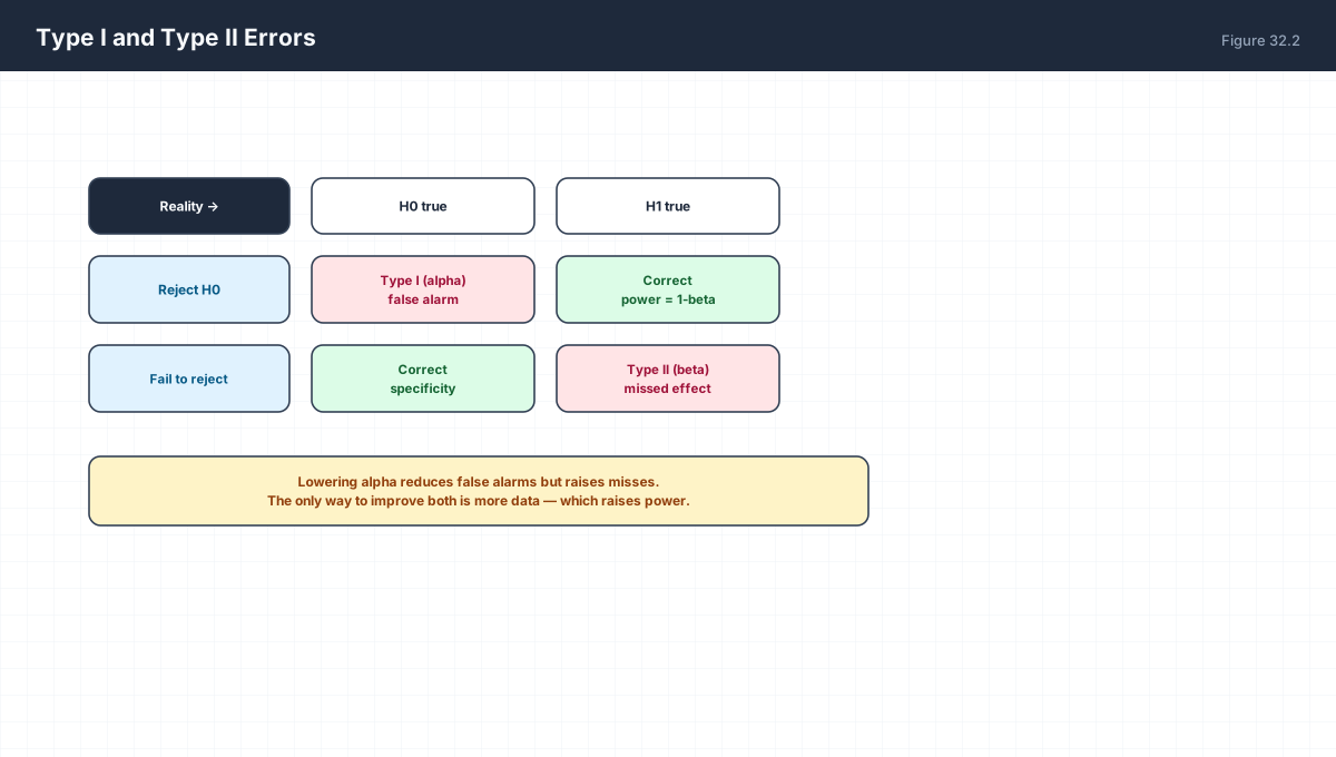
- Explain the difference between Type I and Type II error.
- Show the expected number of false positives under multiplicity.
- Construct and interpret a confidence interval correctly.
- Distinguish statistical from practical significance.
- Report an effect size alongside a p-value.
2. The Logic of the Null
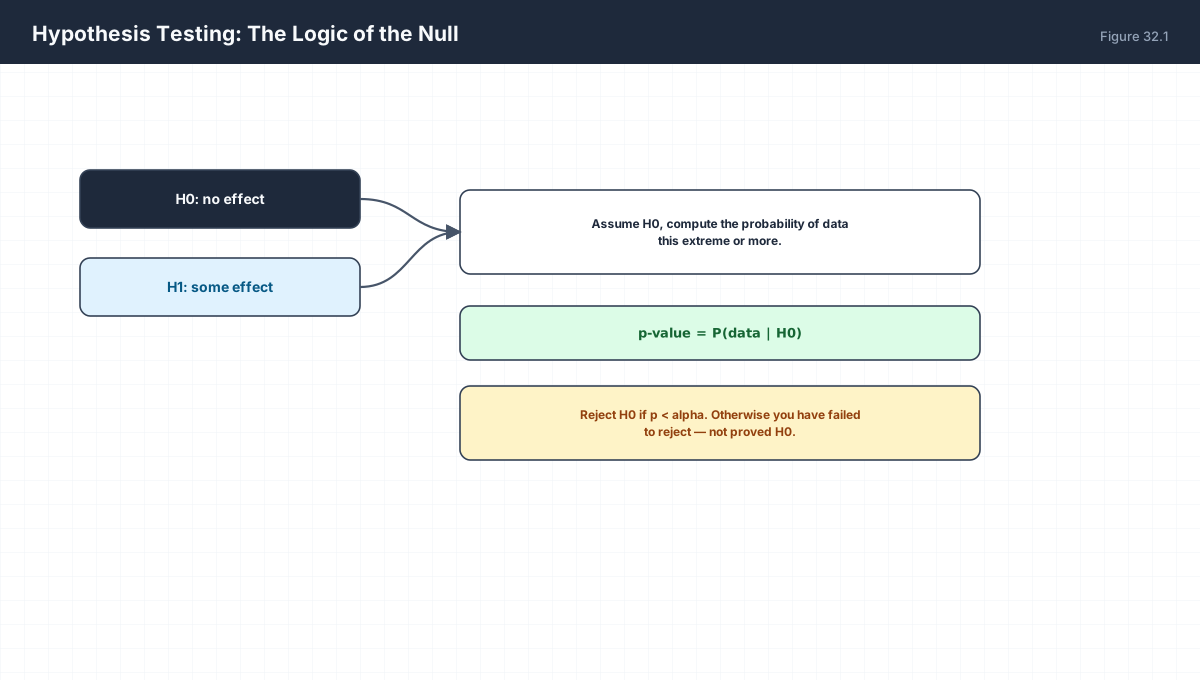
H0: no effect        H1: some effect

p-value = P(data at least as extreme | H0)

Reject H0 if p < alpha (conventionally 0.05).
Fail to reject  !=  prove H0.
import numpy as np
from math import erf, sqrt

rng = np.random.default_rng(0)

# does a new feature improve accuracy?
baseline = rng.binomial(1, 0.70, 1000)
new      = rng.binomial(1, 0.73, 1000)

diff = new.mean() - baseline.mean()
se = np.sqrt(baseline.var() / 1000 + new.var() / 1000)
z = diff / se

normal_cdf = lambda x: 0.5 * (1 + erf(x / sqrt(2)))
p = 2 * (1 - normal_cdf(abs(z)))          # two-sided

print(f"baseline {baseline.mean():.3f}  new {new.mean():.3f}  diff {diff:+.3f}")
print(f"z = {z:.3f}   p-value = {p:.4f}")
print("significant at 0.05:", p < 0.05)
The p-value answers: if the new feature did nothing, how often would a difference this large appear by chance? It does not answer whether the feature works, nor how large the effect is.
3. Two Ways to Be Wrong
| Term | Symbol | Given By |
|---|---|---|
| Significance level | α | You choose it |
| Power | 1 − β | Effect size, variance, and n |
| Minimum detectable effect | δ | Inverse function of n |
import numpy as np
from math import erf, sqrt

normal_cdf = lambda x: 0.5 * (1 + erf(x / sqrt(2)))
rng = np.random.default_rng(1)

def power(effect, n, sigma=1.0, alpha=0.05):
    """Approximate two-sided power for a mean difference."""
    se = sigma * np.sqrt(2 / n)
    crit = 1.959963985 * se
    return 1 - normal_cdf((crit - effect) / se) + normal_cdf((-crit - effect) / se)

for n in (100, 1000, 10000):
    print(f"n={n:6d}  power to detect effect 0.1: {power(0.1, n):.3f}")
Power is the number that makes an experiment worth running. A study with 20% power has an 80% chance of missing a real effect, and a non-significant result from such a study carries almost no information.
4. Multiplicity
import numpy as np

rng = np.random.default_rng(2)

# 20 A/B tests on a metric with no real effect anywhere
n_tests = 20
n = 500
false_positives = 0
for _ in range(2000):
    a = rng.binomial(1, 0.5, n)
    b = rng.binomial(1, 0.5, n)
    se = np.sqrt(a.var()/n + b.var()/n)
    z = (b.mean() - a.mean()) / se
    if abs(z) > 1.959963985:
        false_positives += 1
print(f"tests with >=1 false positive: {false_positives/2000:.3f}")
print("theory: 1 - 0.95^20 =", round(1 - 0.95 ** 20, 3))

# Bonferroni: divide alpha by the number of tests
print("Bonferroni threshold:", 0.05 / n_tests)
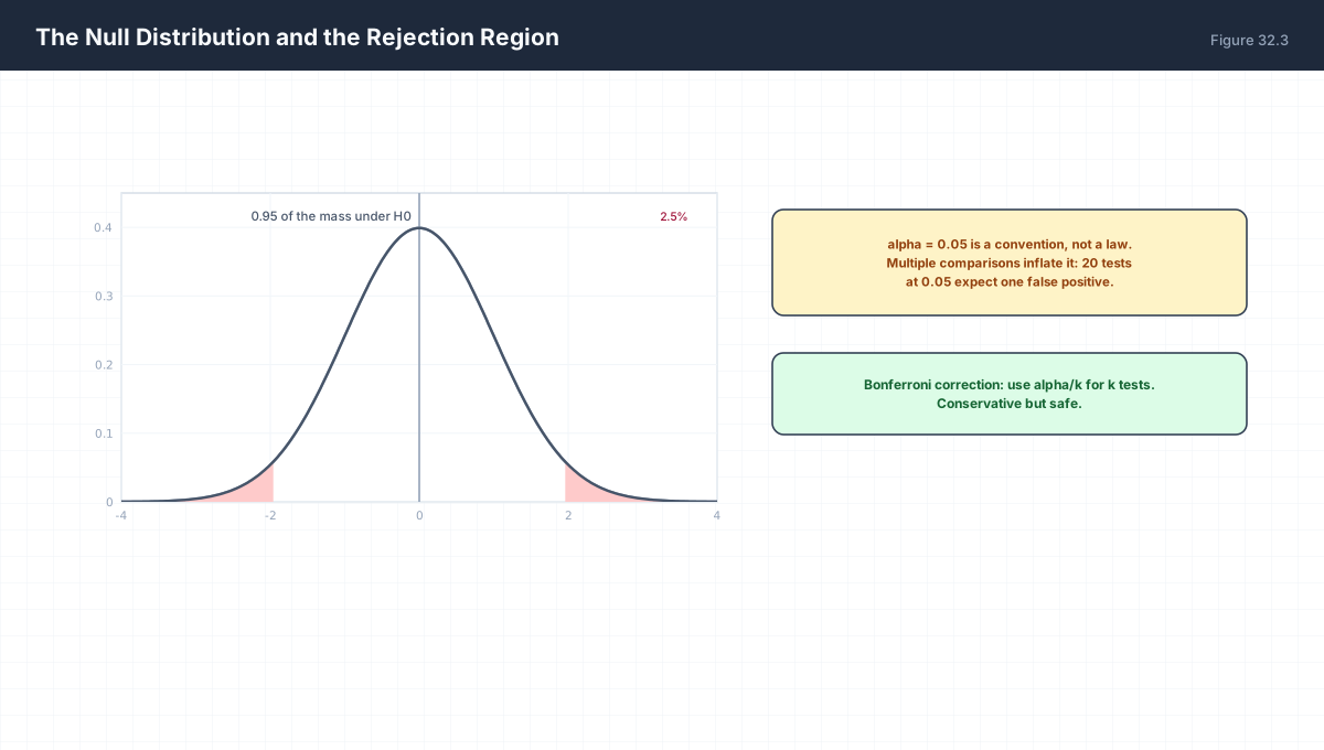
Twenty independent tests at α = 0.05 give a 64% chance of at least one false positive — computed as 1 − 0.95²⁰. This is why tuning many hyperparameters and reporting the best is a form of overfitting: you are selecting on noise.
5. Confidence Intervals
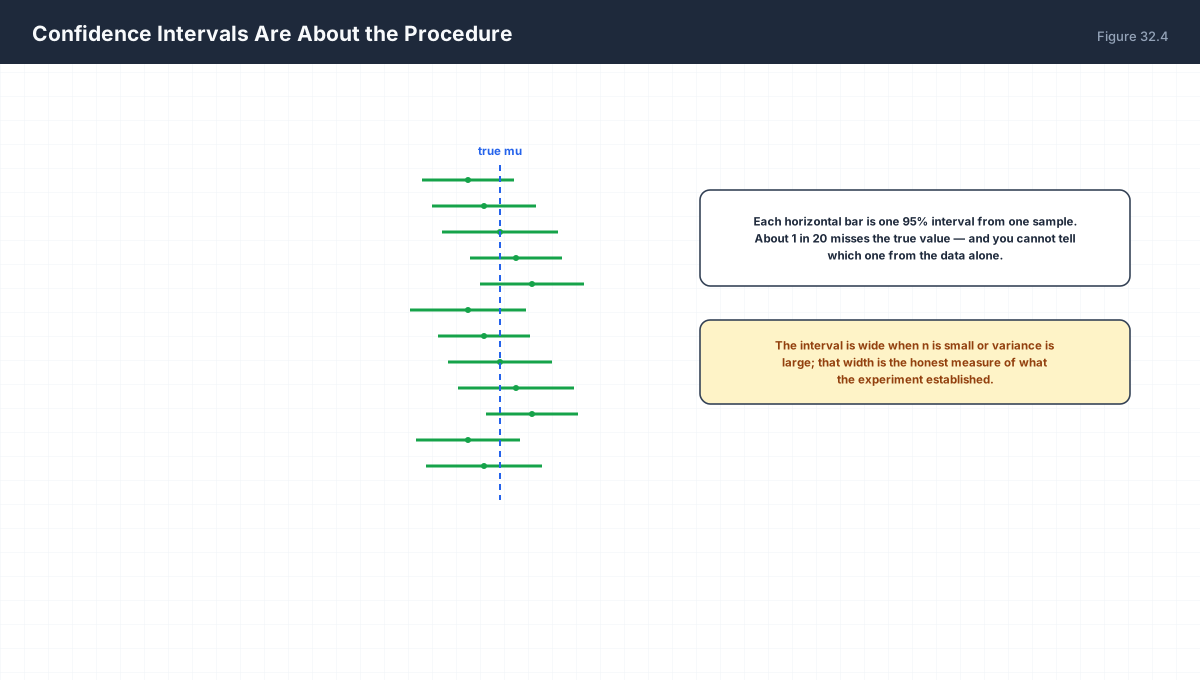
CI = estimate +/- z * SE

95% interval means: if you repeated the experiment many times,
95% of the intervals built this way would contain the true value.
It does NOT mean "95% chance the true value is in this interval"
once the interval is computed — the value is either in it or not.
import numpy as np

rng = np.random.default_rng(3)
true_mu = 5.0
cover = 0
trials = 5000
for _ in range(trials):
    s = rng.normal(true_mu, 1.0, 100)
    lo = s.mean() - 1.959963985 * 1.0 / np.sqrt(100)
    hi = s.mean() + 1.959963985 * 1.0 / np.sqrt(100)
    cover += (lo <= true_mu <= hi)
print(f"coverage across {trials} experiments: {cover/trials:.3f}")
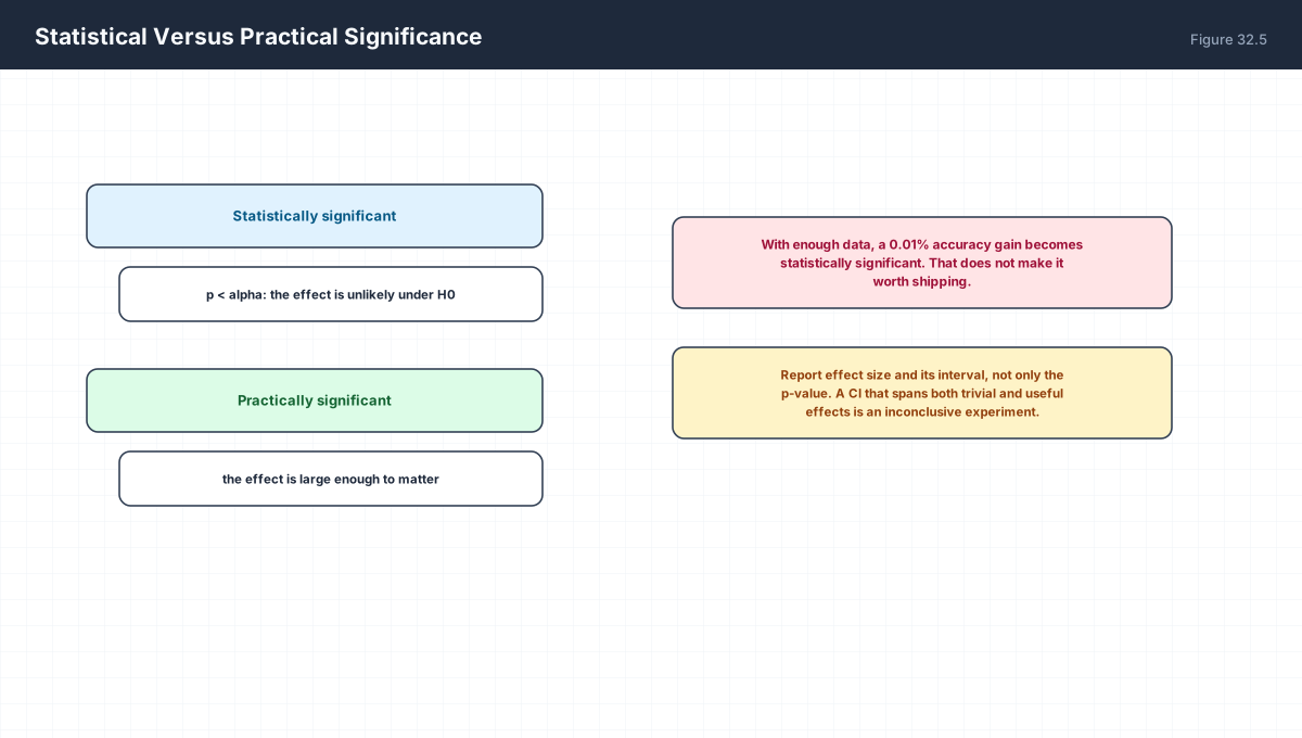
The interval carries more information than the p-value because it shows the magnitude and its uncertainty together. A CI that spans both trivially small and usefully large effects is an inconclusive experiment, and no p-value threshold repairs that.
6. Statistical Versus Practical Significance
| Report | Tells You |
|---|---|
| p-value only | Whether the effect is distinguishable from zero |
| Effect size + CI | How large, and how precisely known |
| n and power | Whether a null result means anything |
7. Worked Examples
7.1 One-sample z-test
sample mean 52, mu0 = 50, sigma = 10, n = 100
z = (52 - 50) / (10/10) = 2.0
two-sided p = 0.0455  ->  just significant at 0.05
7.2 Required sample size
To detect effect d with sigma = 1 at 80% power, alpha 0.05:
n ≈ 16 / d^2
d = 0.1 -> n ≈ 1600
d = 0.5 -> n ≈ 64
7.3 Bonferroni
20 tests, family-wise alpha 0.05
per-test threshold = 0.05/20 = 0.0025
7.4 Interval width
CI half-width = 1.96 sigma / sqrt(n)
To halve it, quadruple n.
7.5 Interpreting a null result
p = 0.4 with n = 30 and power 0.2
This is not evidence of no effect — it is an underpowered test.
8. Verify It in Python
import numpy as np
from math import erf, sqrt

ncdf = lambda x: 0.5 * (1 + erf(x / sqrt(2)))
rng = np.random.default_rng(0)

# --- 1. z-test and p-value ---------------------------------------
a = rng.binomial(1, 0.5, 500)
b = rng.binomial(1, 0.5, 500)
se = np.sqrt(a.var()/len(a) + b.var()/len(b))
z = (b.mean() - a.mean()) / se
p = 2 * (1 - ncdf(abs(z)))
assert 0 <= p <= 1
print(f"z={z:.3f}  p={p:.4f}")

# --- 2. Type I rate under the null -------------------------------
fp = 0
for _ in range(2000):
    x = rng.binomial(1, .5, 300); y = rng.binomial(1, .5, 300)
    s = np.sqrt(x.var()/300 + y.var()/300)
    if abs((y.mean()-x.mean())/s) > 1.959963985:
        fp += 1
rate = fp / 2000
assert 0.02 < rate < 0.08
print(f"Type I rate at alpha=0.05: {rate:.4f}")

# --- 3. multiplicity inflates it --------------------------------
assert 1 - 0.95 ** 20 > 0.6
print("family-wise error for 20 tests:", round(1 - 0.95**20, 3))

# --- 4. power grows with n --------------------------------------
def power(effect, n, sigma=1.0):
    se = sigma * np.sqrt(2 / n)
    crit = 1.959963985 * se
    return 1 - ncdf((crit - effect) / se) + ncdf((-crit - effect) / se)

assert power(0.3, 100) < power(0.3, 1000)
print("power at n=100, 1000:", round(power(0.3,100),3), round(power(0.3,1000),3))

# --- 5. CI coverage is 95% --------------------------------------
cover = 0
for _ in range(4000):
    s = rng.normal(5.0, 1.0, 100)
    lo = s.mean() - 1.959963985 / 10
    hi = s.mean() + 1.959963985 / 10
    cover += (lo <= 5.0 <= hi)
assert abs(cover/4000 - 0.95) < 0.02
print("empirical CI coverage:", round(cover/4000, 4))

# --- 6. CI width scales as 1/sqrt(n) ---------------------------
w100 = 2 * 1.959963985 / np.sqrt(100)
w400 = 2 * 1.959963985 / np.sqrt(400)
assert np.isclose(w100 / w400, 2.0)
print("quadrupling n halves the CI width")

# --- 7. Bonferroni threshold -----------------------------------
assert np.isclose(0.05 / 20, 0.0025)
print("Bonferroni threshold for 20 tests:", 0.05/20)
print("all assertions passed")
9. Practice Questions
- State H₀ and H₁ for a test of whether accuracy improved.
- Define the p-value precisely and state what it is not.
- Distinguish Type I and Type II error with an example each.
- Explain why lowering α raises β.
- Compute the family-wise error rate for 10 tests at α = 0.05.
- State the Bonferroni threshold for 25 tests.
- Interpret a 95% confidence interval correctly in one sentence.
- What does a non-significant result from an underpowered study tell you?
- Give an example where an effect is statistically but not practically significant.
- Why does quadrupling n halve a confidence interval's width?
10. Official References & Further Reading
Continue the Course
- Course Index: AI Mathematics Masterclass — All 48 Chapters
- Previous Chapter: Chapter 31: Descriptive Statistics & Data Summarization
- Next Chapter: Chapter 33: Correlation & Regression Mathematics
- Related Series: PyTorch Engineering Masterclass — All 16 Modules