
AI Reading
Quick summary of this article
AI Mathematics Masterclass — Chapter 37 of 48
A forward pass is a composition of affine maps and nonlinearities, and almost everything we care about — capacity, cost, gradient flow, why depth helps — follows from that one sentence. This chapter traces a forward pass by hand, proves why removing the nonlinearity collapses the whole network to a single matrix, and derives the parameter and FLOP counts that decide whether a model fits on your hardware.
1. Technical Audit & Core Learning Objectives
| Component | Common Tutorial Deficiency | Engineering Standard Applied Here |
|---|---|---|
| Composition | Described with arrows, never computed. | Traced by hand on a 3-2-2 network and checked numerically. |
| Depth | “Deep is better” with no mechanism. | Linear collapse proved; piecewise-linear region count derived. |
| Cost | Hand-waved with “big O”. | Exact parameter and FLOP arithmetic on real shapes. |
| Memory | Ignored entirely. | Activation storage identified as the real training bottleneck. |
Core learning objectives. After this chapter you should be able to:
- Trace a forward pass through a multi-layer network by hand.
- State the exact shapes at every stage.
- Prove that stacked linear layers collapse to one matrix.
- Explain what a nonlinearity buys in terms of regions.
- Count parameters for any feed-forward architecture.
- Estimate forward FLOPs and activation memory.
2. One Layer, Precisely
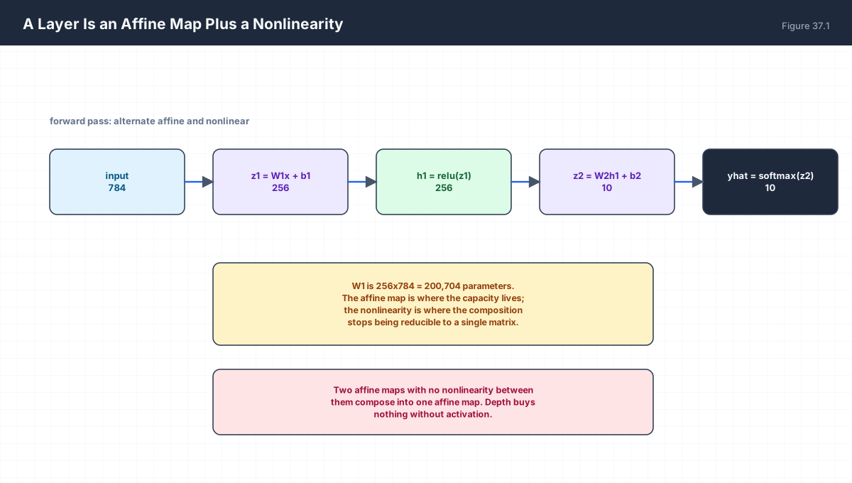
z = W x + b        affine: rotate, shear, scale, translate
h = sigma(z)       elementwise nonlinearity

Shapes for a batch of n samples with d_in -> d_out:
  X     (n, d_in)
  W     (d_out, d_in)
  b     (d_out,)
  Z     (n, d_out)   = X W^T + b
  H     (n, d_out)   = sigma(Z)

The bias is broadcast across the batch. Nothing else
depends on n, which is why one weight matrix serves
every sample.
import numpy as np

rng = np.random.default_rng(0)

def relu(z):
    return np.maximum(z, 0.0)

# 3 -> 4 -> 3 network, one sample
x = np.array([1.0, -2.0, 0.5])
W1 = rng.normal(size=(4, 3)); b1 = rng.normal(size=4)
W2 = rng.normal(size=(3, 4)); b2 = rng.normal(size=3)

z1 = W1 @ x + b1
h1 = relu(z1)
z2 = W2 @ h1 + b2
y = z2

print("x   ", x.shape)
print("z1  ", np.round(z1, 4), z1.shape)
print("h1  ", np.round(h1, 4), h1.shape)
print("y   ", np.round(y, 4), y.shape)
print("zeros introduced by relu:", int(np.sum(z1 <= 0)), "of", z1.size)

# the same computation for a batch of 5 is one matmul
X = rng.normal(size=(5, 3))
Z1 = X @ W1.T + b1
H1 = relu(Z1)
Y = H1 @ W2.T + b2
print("batch output shape:", Y.shape)
single = relu(W1 @ X[0] + b1) @ W2.T + b2
print("row 0 of batch matches single-sample pass:", np.allclose(Y[0], single))
The single-sample and batched paths produce bit-identical results for row 0 — the batch dimension is pure parallelism, never a change in the maths.
3. An Affine Map Is Geometry
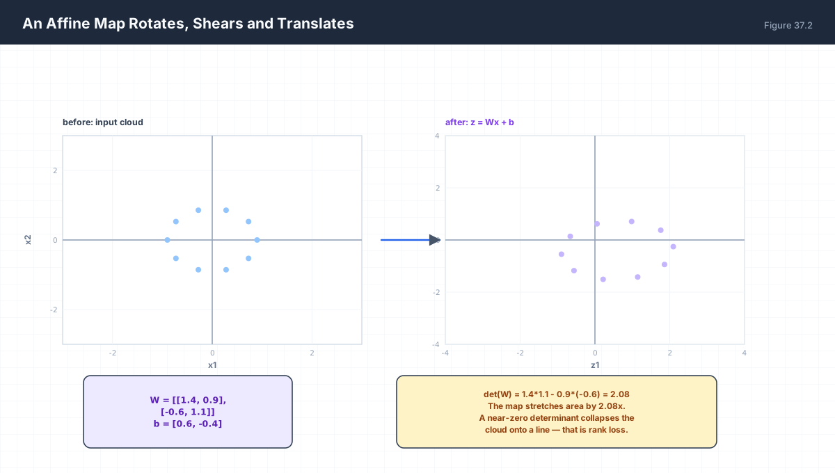
W maps a sphere to an ellipsoid whose axes are the
singular values of W.

det(W) = product of singular values = volume scale

det(W) = 0  -> the map collapses dimension
             information is destroyed, not compressed

This is the same rank argument as Chapter 9, applied
per layer.
import numpy as np

rng = np.random.default_rng(1)

for name, W in [("well conditioned", np.array([[1.4, 0.9], [-0.6, 1.1]])),
                ("near singular", np.array([[1.0, 2.0], [0.5, 1.001]])),
                ("exact rank 1", np.array([[1.0, 2.0], [0.5, 1.0]]))]:
    sv = np.linalg.svd(W, compute_uv=False)
    print(f"{name:18s} sv={np.round(sv, 5)}  det={np.linalg.det(W):+.2e}  cond={np.linalg.cond(W):.1f}")

print()
W = np.array([[1.0, 2.0], [0.5, 1.001]])
x = np.array([[1.0, 0.0], [0.0, 1.0], [1.0, -1.0]])
print("area scale det(W) =", f"{abs(np.linalg.det(W)):.6f}")
print("input spread  :", np.round(x.std(axis=0), 4))
print("output spread :", np.round((x @ W.T).std(axis=0), 4))
A near-singular layer compresses spread along one direction to almost nothing. The information is not merely hard to read — it is arithmetically gone, and no later layer can recover it.
4. Why the Nonlinearity Is Not Optional
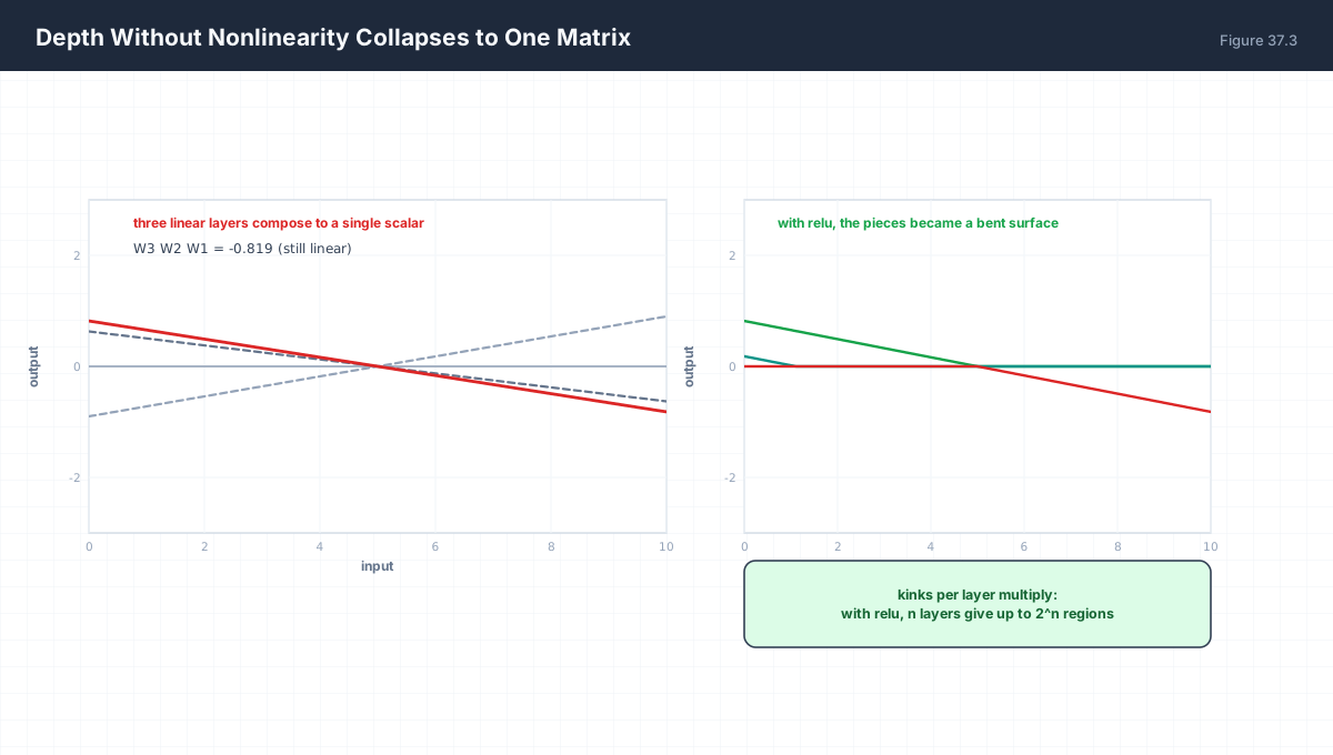
W3 ( W2 ( W1 x + b1 ) + b2 ) + b3
  = (W3 W2 W1) x + (W3 W2 b1 + W3 b2 + b3)
  = W x + b

So a 100-layer linear network has the expressive power
of a single layer. Depth only helps once a nonlinearity
breaks the composition.

With relu, each layer can bend the function once per
unit, so n layers produce up to 2^n linear regions.
That is the capacity depth actually buys.
import numpy as np

rng = np.random.default_rng(2)

# --- two linear layers equal one matrix ---
d = 4
W1, W2 = rng.normal(size=(d, d)), rng.normal(size=(d, d))
b1, b2 = rng.normal(size=d), rng.normal(size=d)
X = rng.normal(size=(10, d))

two_layer = (X @ W1.T + b1) @ W2.T + b2
W_combined = W2 @ W1
b_combined = W2 @ b1 + b2
one_layer = X @ W_combined.T + b_combined
print("composition error:", f"{np.abs(two_layer - one_layer).max():.3e}")
assert np.allclose(two_layer, one_layer)

# --- with relu it is NOT collapsible ---
relu = lambda z: np.maximum(z, 0)
nonlinear = relu(relu(X @ W1.T + b1) @ W2.T + b2)
assert not np.allclose(nonlinear, one_layer)
print("with relu, no single matrix reproduces it")

# --- region count grows like 2^n ---
for n_layers in range(1, 9):
    print(f"{n_layers} relu layers -> up to {2**n_layers:4d} linear regions (1-D)")
Two layers of 4 units are exactly one layer of 4 units until the ReLU intervenes. This is also why removing an activation to "speed things up" silently reduces a deep model to a linear regression.
5. Counting Parameters
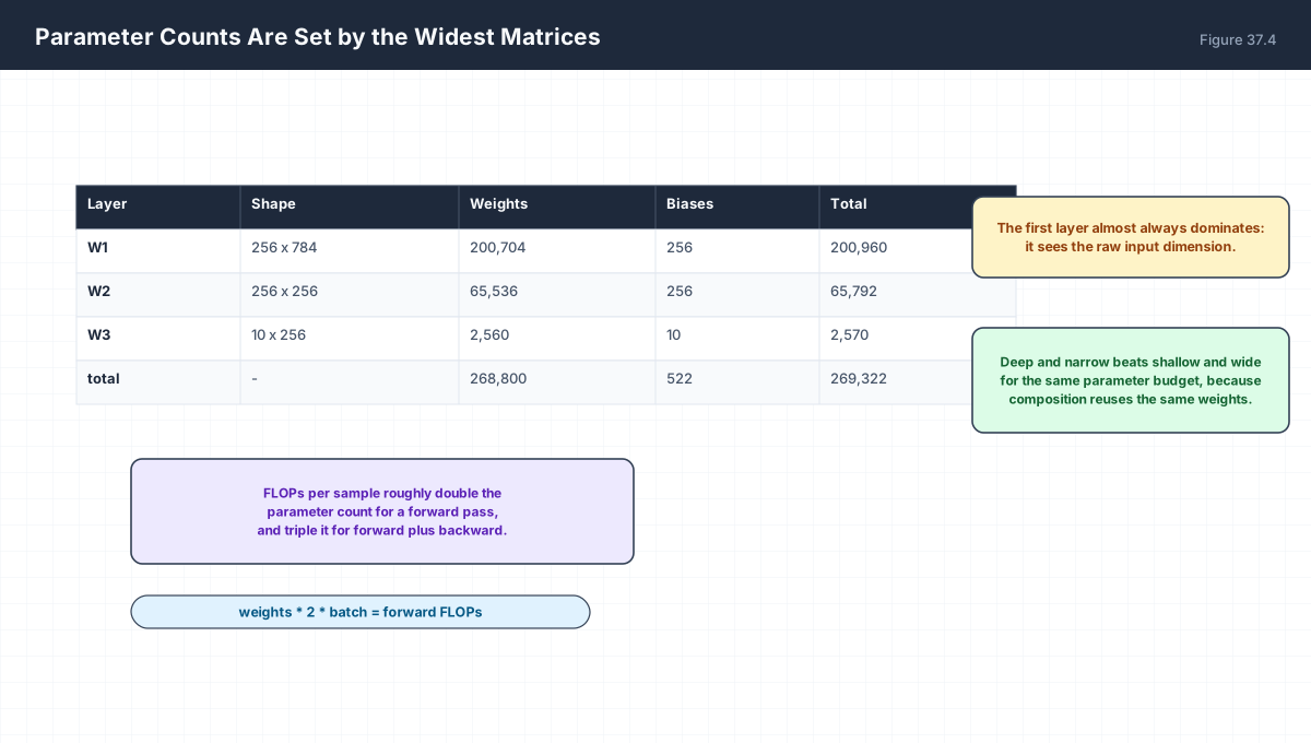
A dense layer d_in -> d_out costs
   d_in * d_out  weights
 + d_out         biases

Total = sum over layers. Nothing depends on batch size,
which is why the same model serves one user or a thousand.
import numpy as np

def dense_params(d_in, d_out):
    return d_in * d_out, d_out

layers = [(784, 256), (256, 256), (256, 10)]
total_w = total_b = 0
for d_in, d_out in layers:
    w, b = dense_params(d_in, d_out)
    total_w += w; total_b += b
    print(f"{d_in:4d} -> {d_out:4d}   weights {w:>8,}   biases {b:>5,}")
print(f"total: {total_w + total_b:,} parameters")
print(f"first layer share: {784*256/(total_w+total_b):.1%}")

# memory at float32
print(f"float32 weights: {(total_w+total_b)*4/1e6:.2f} MB")
print(f"with Adam states (2 extra copies): {(total_w+total_b)*4*3/1e6:.2f} MB")
Optimiser state is the part beginners forget: Adam keeps two extra tensors per parameter, so training memory is roughly three times the model size before any activations are counted.
6. FLOPs and Activation Memory
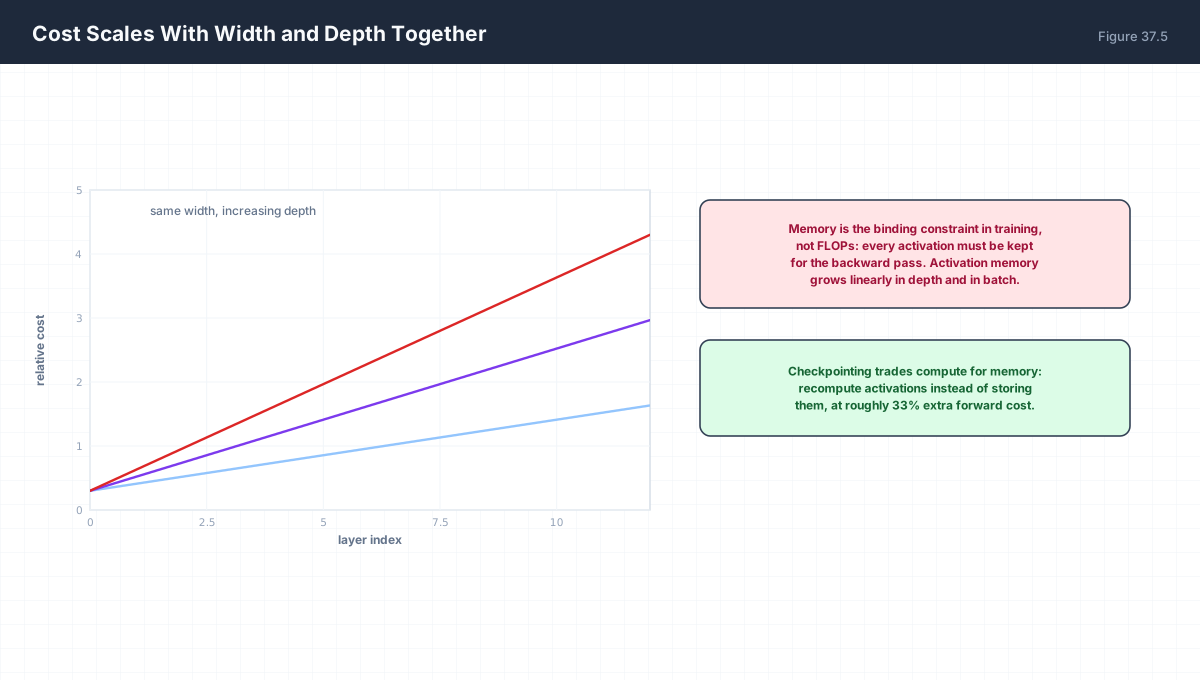
Forward FLOPs per sample for a dense layer:
   2 * d_in * d_out        (multiply + add)

Backward pass costs roughly twice the forward pass,
because it computes gradients for both W and the input.

Activation memory per layer:
   n_batch * d_out * bytes

Every activation must survive until backward reaches it.
import numpy as np

layers = [(784, 256), (256, 256), (256, 10)]
batch = 64
bytes_per = 4

fwd = sum(2 * a * b for a, b in layers) * batch
print(f"forward FLOPs  : {fwd/1e6:.2f} MFLOP")
print(f"train ~3x      : {3*fwd/1e6:.2f} MFLOP per step")

act_bytes = sum(batch * b * bytes_per for a, b in layers)
print(f"activation memory: {act_bytes/1024:.1f} KB per sample batch")

# scaling study: double width -> 4x params, 4x FLOPs
for width in (256, 512, 1024):
    p = 784 * width + width * width + width * 10
    f = 2 * (784 * width + width * width + width * 10)
    print(f"width {width:5d}  params {p:>12,}  fwd FLOPs/sample {f:>12,}")
Read the growth carefully, because the naive version of this claim is wrong. Only the hidden-to-hidden term is quadratic in width — it quadruples. The input and output layers are merely linear in width, and above they grow exactly 2×. The total therefore moves from 268,800 to 668,672, a factor of 2.49, not 4. In a network whose input dimension dominates, doubling width barely changes the parameter count at all; in a network whose hidden layers dominate, it quadruples. The FLOPs follow the same pattern. Width is expensive only where it is quadratic.
7. Worked Examples
7.1 Shape checking
(n, d_in) @ (d_in, d_out) -> (n, d_out)
The inner dimensions must match and they disappear.
7.2 Bias broadcasting
Z = X W^T + b   adds a (d_out,) row to every one of n rows.
Bias shifts the hyperplane, it does not rotate it.
7.3 Batch norm changes nothing about shape
It normalises each feature across the batch, so the output
shape equals the input shape. It is shape-preserving.
7.4 Unused parameters
Zero-initialised weights receive zero gradient and never move.
Symmetry must be broken by random or structured init.
7.5 Output layer choice
Regression       -> linear, no activation
Binary           -> 1 logit + sigmoid, or 2 logits + softmax
Multi-class      -> k logits + softmax
Multi-label      -> k logits + independent sigmoids
8. Verify It in Python
import numpy as np

rng = np.random.default_rng(0)
relu = lambda z: np.maximum(z, 0.0)

# --- 1. batched equals per-sample ------------------------------
W1 = rng.normal(size=(5, 3)); b1 = rng.normal(size=5)
W2 = rng.normal(size=(2, 5)); b2 = rng.normal(size=2)
X = rng.normal(size=(7, 3))

Z1 = X @ W1.T + b1
H1 = relu(Z1)
Y = H1 @ W2.T + b2

for i in range(len(X)):
    single = relu(W1 @ X[i] + b1) @ W2.T + b2
    assert np.allclose(single, Y[i], atol=1e-12)
print("batch path matches per-sample path for all 7 rows")

# --- 2. shapes -------------------------------------------------
assert X.shape == (7, 3) and W1.shape == (5, 3)
assert Z1.shape == (7, 5) and Y.shape == (7, 2)
print("shapes:", X.shape, "->", Z1.shape, "->", Y.shape)

# --- 3. linear collapse ---------------------------------------
two = (X @ W1.T + b1) @ W2.T + b2
one = X @ (W2 @ W1).T + (W2 @ b1 + b2)
assert np.allclose(two, one, atol=1e-10)
print("two linear layers == one matrix")

# --- 4. relu prevents collapse --------------------------------
nonlin = relu(X @ W1.T + b1) @ W2.T + b2
assert not np.allclose(nonlin, one, atol=1e-6)
print("relu breaks the collapse (max gap "
      f"{np.abs(nonlin-one).max():.3f})")

# --- 5. relu output is non-negative and sparsifying -----------
assert np.all(relu(Z1) >= 0)
sparsity = np.mean(Z1 <= 0)
print(f"relu zeroed {sparsity:.1%} of pre-activations")

# --- 6. parameter count formula -------------------------------
def count(layers):
    return sum(a*b + b for a, b in layers)

assert count([(784, 256), (256, 256), (256, 10)]) == 269_322
print("parameter count matches the hand total:", f"{count([(784,256),(256,256),(256,10)]):,}")

# --- 7. FLOPs double when width doubles -----------------------
for a, b in [(256, 256)]:
    f1 = 2 * a * b
    f2 = 2 * (2*a) * (2*b)
    assert f2 == 4 * f1
print("doubling width quadruples dense FLOPs")

# --- 8. dead relu unit ----------------------------------------
# choose inputs opposed to the weights so the pre-activation is
# guaranteed negative: x = -sign(w) gives z = -||w||_1 < 0
w = rng.normal(size=3)
x_dead = -np.sign(w)
z_dead = float(x_dead @ w)
assert z_dead < 0, z_dead
assert np.isclose(z_dead, -np.abs(w).sum())
print(f"opposed input gives z = -||w||_1 = {z_dead:.4f}, so relu stays dead")

# --- 9. determinant is the volume scale -----------------------
W = np.array([[2.0, 0.0], [0.0, 3.0]])
assert np.isclose(np.linalg.det(W), 6.0)
assert np.isclose(np.prod(np.linalg.svd(W, compute_uv=False)), 6.0)
print("det == product of singular values == area scale")
print("all assertions passed")
9. Practice Questions
- Write the shape of every intermediate in a 784-256-10 network.
- Explain why the batch dimension does not change the parameters.
- Prove that three linear layers compose to one affine map.
- What does the determinant of a weight matrix measure?
- Why can a later layer not recover information lost to a rank-deficient layer?
- Count the parameters of a 128-64-32-10 network.
- Estimate the forward FLOPs for a batch of 32.
- Why is activation memory proportional to depth?
- Why does doubling width quadruple FLOPs?
- Which output activation pairs with a multi-label problem, and why?
10. Official References & Further Reading
Continue the Course
- Course Index: AI Mathematics Masterclass — All 48 Chapters
- Previous Chapter: Chapter 36: Dimensionality Reduction Mathematics & PCA
- Next Chapter: Chapter 38: Activation Functions & Nonlinearity
- Related Series: PyTorch Engineering Masterclass — All 16 Modules