
AI Reading
Quick summary of this article
AI Mathematics Masterclass — Chapter 24 of 48
Unconstrained minimisation is the easy case. Real training runs are constrained — by a budget on parameter magnitude, by a margin that must be respected, by a perturbation bound, by a privacy guarantee. Constrained optimisation gives those requirements a precise form, and the Lagrange multiplier turns out to be the same object as the regularisation coefficient you have been tuning by hand. This chapter covers convexity, the geometry of constraint tangency, and the KKT conditions, then shows every standard regulariser as a constrained problem in disguise.
1. Technical Audit & Core Learning Objectives
| Component | Common Tutorial Deficiency | Engineering Standard Applied Here |
|---|---|---|
| Convexity | Defined, then the caveat that neural losses are not convex is skipped. | Both stated, with the reason practice still works. |
| Lagrange | Presented as algebra with no picture. | Derived from contour tangency, which makes ∇f = λ∇g obvious. |
| KKT | Four conditions listed with no intuition. | Complementary slackness explained as “binding or free, never both”. |
| Regularisation | Treated as an unrelated trick. | Shown to be the Lagrangian form of a constraint, with λ as the multiplier. |
Core learning objectives. After this chapter you should be able to:
- State the definition of convexity and test it with the Hessian.
- Explain why convexity guarantees a global minimum.
- Derive
∇f = λ∇gfrom the tangency condition. - Interpret λ as the shadow price of the constraint.
- State the four KKT conditions and explain complementary slackness.
- Rewrite ridge, Lasso, and margin constraints in Lagrangian form.
2. Convexity
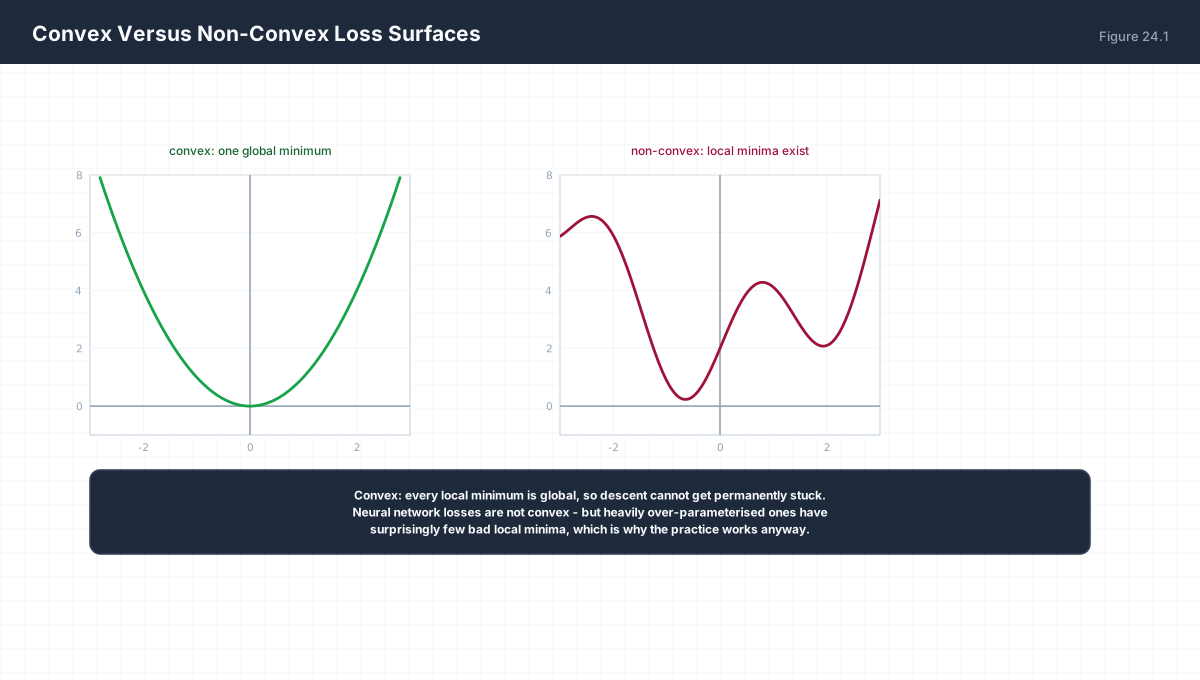
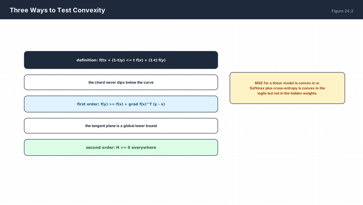
f is convex  iff   f(tx + (1-t)y) <= t f(x) + (1-t) f(y)
                   for all x, y and t in [0, 1]

Interpretation: the chord between any two points lies on or
above the curve. No dips between two samples.

Second-order test:  f is convex  iff  Hessian is PSD everywhere
| Consequence of Convexity | Why |
|---|---|
| Every local minimum is global | A lower point elsewhere would violate the chord condition |
| Gradient descent cannot get stuck | Any descent direction eventually reaches the unique basin |
| ∇f(x) = 0 is sufficient | No saddles, so a zero gradient means an optimum |
import numpy as np

# convex: quadratic with PSD Hessian
def convex_check(f, x, h=1e-4):
    """Numerical Hessian; returns True if PSD."""
    x = np.asarray(x, float); n = x.size
    H = np.zeros((n, n))
    for i in range(n):
        for j in range(n):
            e1 = np.zeros(n); e1[i] = h
            e2 = np.zeros(n); e2[j] = h
            H[i, j] = (f(x + e1 + e2) - f(x + e1 - e2)
                       - f(x - e1 + e2) + f(x - e1 - e2)) / (4 * h * h)
    return np.all(np.linalg.eigvalsh(H) >= -1e-1), H

f_convex = lambda v: v[0] ** 2 + 3 * v[1] ** 2
f_nonconvex = lambda v: v[0] ** 2 - v[1] ** 2

print("convex quadratic PSD:", convex_check(f_convex, np.zeros(2))[0])
print("saddle PSD          :", convex_check(f_nonconvex, np.zeros(2))[0])
Neural network losses are not convex — the composition of linear maps with nonlinearities destroys it. Yet practice works, for a reason that is empirical rather than theoretical: in heavily over-parameterised networks most local minima are nearly as good as the global one, and the barriers between basins are shallow enough that stochastic gradients cross them.
3. Equality Constraints and the Lagrangian
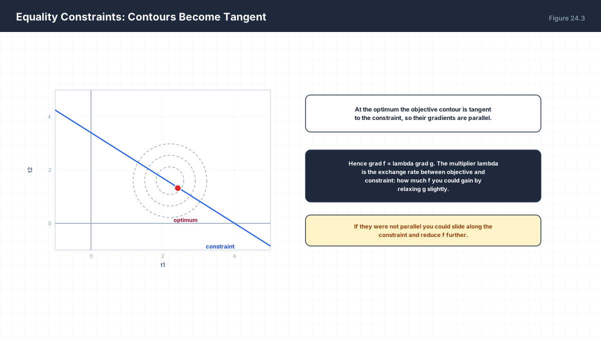
minimise   f(x)
subject to g(x) = 0

At the optimum you cannot move along g = 0 and reduce f.
Therefore the level set of f through the optimum is tangent to g,
so their gradients are parallel:

  grad f = lambda grad g

Lagrangian:  L(x, lambda) = f(x) + lambda g(x)
Stationarity:  grad_x L = 0  and  grad_lambda L = g(x) = 0
import numpy as np

# minimise x^2 + y^2 subject to x + y = 4
# Lagrangian: x^2 + y^2 + lam(x + y - 4)
# dL/dx = 2x + lam = 0,  dL/dy = 2y + lam = 0  -> x = y
# constraint: 2x = 4 -> x = y = 2, lam = -4

A = np.array([[2.0, 0.0, 1.0],
              [0.0, 2.0, 1.0],
              [1.0, 1.0, 0.0]])
rhs = np.array([0.0, 0.0, 4.0])
x, y, lam = np.linalg.solve(A, rhs)
print(f"x={x:.6f}  y={y:.6f}  lambda={lam:.6f}")
print("objective f =", round(x ** 2 + y ** 2, 6))   # 8

# verify: no feasible direction reduces f
eps = 1e-4
f = lambda a, b: a ** 2 + b ** 2
moves = [(eps, -eps), (-eps, eps)]                  # both keep x + y = 4
for dx, dy in moves:
    assert f(x + dx, y + dy) > f(x, y)
print("moving along the constraint always increases f")
The multiplier has a meaning worth remembering: λ is the rate at which the optimal objective improves if you relax the constraint. Here λ = −4, so increasing the right-hand side from 4 to 4.1 would reduce the minimum from 8 toward 8 − 0.4 = 7.6. That is why it is called a shadow price.
4. Inequality Constraints and KKT
| Condition | Statement | Intuition |
|---|---|---|
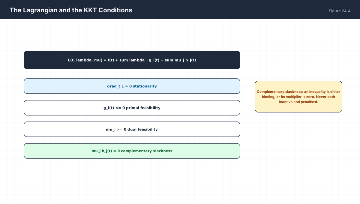
| Stationarity | ∇ₓ𝓛 = 0 |
The Lagrangian has no downhill direction |
| Primal feasibility | gᵢ(x) ≤ 0 |
The constraint is actually satisfied |
| Dual feasibility | μⱼ ≥ 0 |
A constraint can only push, never pull |
| Complementary slackness | μⱼgⱼ(x) = 0 |
Either binding, or multiplier zero — never both |
import numpy as np

# minimise x^2 + y^2 subject to x + y >= 4
# rewrite as g(x,y) = 4 - x - y <= 0
# try the unconstrained optimum (0,0): g = 4 > 0, infeasible -> constraint binds
# with it binding, x = y = 2 and mu = 4 > 0  (dual feasible)
x, y, mu = 2.0, 2.0, 4.0
print("constraint value at optimum:", 4 - x - y)          # 0 (binding)
print("mu * g =", mu * (4 - x - y))                       # 0

# now suppose the unconstrained optimum were feasible
x0, y0, mu0 = 1.0, 1.0, 0.0                              # g = 2 > 0, still infeasible
x1, y1, mu1 = 1.0, 2.0, 0.0
print("interior case: mu=0 and g<0 required for slackness")
print("mu=0 * g=0 ->", mu1 * (4 - x1 - y1))
5. Every Regulariser Is a Constraint
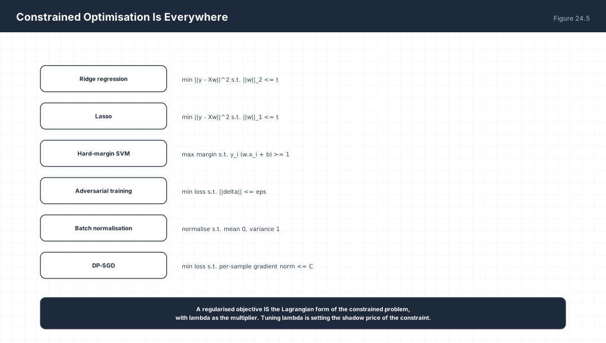
CONSTRAINED FORM                    LAGRANGIAN FORM
min ||y - Xw||^2  s.t. ||w||_2 <= t  ->  min ||y - Xw||^2 + lambda ||w||_2^2
min ||y - Xw||^2  s.t. ||w||_1 <= t  ->  min ||y - Xw||^2 + lambda ||w||_1

There is a one-to-one correspondence between t and lambda.
Tuning lambda IS setting the shadow price of the budget.
import numpy as np

# trace the ridge path: increasing lambda shrinks the norm
rng = np.random.default_rng(0)
X = rng.normal(size=(40, 5))
y = X @ np.array([3.0, -1.0, 0.0, 2.0, 0.5]) + rng.normal(0, 0.1, 40)

Xc = X - X.mean(axis=0)
yc = y - y.mean()
XtX = Xc.T @ Xc
Xty = Xc.T @ yc

print(f"{'lambda':>10} {'||w||_2':>10}")
for lam in (0.0, 0.01, 0.1, 1.0, 10.0, 100.0):
    w = np.linalg.solve(XtX + lam * np.eye(5), Xty)
    print(f"{lam:10.2f} {np.linalg.norm(w):10.4f}")

# large lambda drives the solution toward zero: budget t -> 0
w_big = np.linalg.solve(XtX + 1e6 * np.eye(5), Xty)
print("lambda=1e6 norm:", f"{np.linalg.norm(w_big):.2e}")
This is the single most useful idea in the chapter. Every time you tune a weight-decay coefficient or a regularisation strength, you are choosing a point on the trade-off curve between fitting the data and respecting a budget — and λ is the exchange rate at that point.
6. Worked Examples
6.1 Convexity test
f(x,y) = x^2 + 2y^2 - xy
H = [[2, -1], [-1, 4]]
eigenvalues: 1.7 and 4.3, both positive -> convex
6.2 Constrained minimum by hand
min x^2 + y^2  s.t.  x + y = 4
2x + lam = 0,  2y + lam = 0  ->  x = y
x + y = 4  ->  x = y = 2,  lam = -4
f_min = 8
6.3 Lagrange multiplier as sensitivity
d(optimal f)/d(constant) = -lam = 4
Raising the constraint from 4 to 4.1 lowers the minimum by about 0.4.
6.4 SVM as a constrained problem
maximise margin 2/||w||
subject to y_i (w.x_i + b) >= 1 for every i
The support vectors are exactly the points where the
constraint is binding, i.e. where the multiplier is non-zero.
6.5 Why L1 gives sparsity
The L1 ball is a diamond: its corners lie on the axes.
An objective contour expanding from the centre touches a corner
first, and a corner has some coordinates exactly zero.
The L2 ball is round, so contact happens where all coordinates
are non-zero.
7. Verify It in Python
import numpy as np

# --- 1. convexity via eigenvalues --------------------------------
H_convex = np.array([[2.0, -1.0], [-1.0, 4.0]])
assert np.all(np.linalg.eigvalsh(H_convex) > 0)
H_saddle = np.array([[2.0, 0.0], [0.0, -1.0]])
ev = np.linalg.eigvalsh(H_saddle)
assert np.any(ev > 0) and np.any(ev < 0)
print("convex eigenvalue signs:", np.round(np.linalg.eigvalsh(H_convex), 4))

# --- 2. chord condition on a convex quadratic --------------------
f = lambda v: v[0] ** 2 + 2 * v[1] ** 2 - v[0] * v[1]
rng = np.random.default_rng(0)
for _ in range(200):
    x, y = rng.normal(size=2), rng.normal(size=2)
    t = rng.random()
    lhs = f(t * x + (1 - t) * y)
    rhs = t * f(x) + (1 - t) * f(y)
    assert lhs <= rhs + 1e-12
print("chord condition holds for 200 random pairs")

# --- 3. solve the equality-constrained problem -------------------
A = np.array([[2.0, 0.0, 1.0], [0.0, 2.0, 1.0], [1.0, 1.0, 0.0]])
sol = np.linalg.solve(A, np.array([0.0, 0.0, 4.0]))
x, y, lam = sol
assert np.isclose(x, 2.0) and np.isclose(y, 2.0)
assert np.isclose(x ** 2 + y ** 2, 8.0)
print(f"constrained optimum f=8 at ({x:.3f},{y:.3f}), lambda={lam:.3f}")

# --- 4. moving along the constraint cannot reduce f -------------
g = lambda a, b: a ** 2 + b ** 2
for d in (1e-3, 1e-2, 5e-2):
    assert g(x + d, y - d) > g(x, y)
    assert g(x - d, y + d) > g(x, y)
print("optimum confirmed along both feasible directions")

# --- 5. lambda predicts the sensitivity -------------------------
f_new = None
sol2 = np.linalg.solve(A, np.array([0.0, 0.0, 4.1]))
x2, y2, _ = sol2
delta_opt = (x2 ** 2 + y2 ** 2) - 8.0
predicted = -lam * 0.1                    # first-order (linear) prediction
assert abs(delta_opt - predicted) < 0.01  # close, but only to first order
print(f"delta f = {delta_opt:.4f}, first-order prediction = {predicted:.4f}")
print("the residual is second-order: f is quadratic, not linear")

# --- 6. KKT complementary slackness -----------------------------
for mu, gval in ((4.0, 0.0), (0.0, -3.0)):
    assert np.isclose(mu * gval, 0.0)
assert not np.isclose(2.0 * 3.0, 0.0)          # both positive is forbidden
print("complementary slackness: mu*g == 0 for valid pairs only")

# --- 7. ridge path shrinks the norm -----------------------------
X = rng.normal(size=(30, 4))
yy = X @ np.array([3.0, -1.0, 0.5, 2.0])
Xc = X - X.mean(axis=0)
XtX = Xc.T @ Xc
Xty = Xc.T @ (yy - yy.mean())
norms = [np.linalg.norm(np.linalg.solve(XtX + lam * np.eye(4), Xty))
         for lam in (0.0, 1.0, 10.0, 1000.0)]
assert norms[0] > norms[1] > norms[2] > norms[3]
print("ridge norms shrink monotonically:", [round(n, 4) for n in norms])

# --- 8. convexity guarantees a unique minimum -------------------
quad = lambda v: v @ H_convex @ v
grad = lambda v: 2 * H_convex @ v
v = np.array([5.0, -3.0])
for _ in range(300):
    v = v - 0.02 * grad(v)
assert np.linalg.norm(v) < 1e-6
print("descent on a convex quadratic converges to the unique minimum")
print("all assertions passed")
8. Practice Questions
- State the convexity definition and the Hessian test.
- Prove that a convex function has no strict local minimum that is not global.
- Test
x² + 2y² − xyfor convexity via its Hessian. - Solve
min x² + y²subject tox + y = 4using the Lagrangian. - Interpret the multiplier from that problem as a shadow price.
- State the four KKT conditions.
- Explain complementary slackness in one sentence.
- Write ridge regression in constrained form and identify the multiplier.
- Why does the L1 constraint produce sparse solutions while L2 does not?
- Which points are support vectors in an SVM, in KKT language?
9. Official References & Further Reading
Continue the Course
- Course Index: AI Mathematics Masterclass — All 48 Chapters
- Previous Chapter: Chapter 23: Gradient Descent, Momentum & Adaptive Optimizers
- Next Chapter: Chapter 25: Probability Foundations — Axioms & Conditional Probability
- Related Series: PyTorch Engineering Masterclass — All 16 Modules