
AI Reading
Quick summary of this article
AI Mathematics Masterclass — Chapter 12 of 48
When a linear system has no exact solution, the right question is not “how do I force one” but “which point in the reachable set is closest to what I want”. That question is answered by orthogonal projection, and its application to over-determined systems is least squares — the closed-form solution to linear regression. This chapter derives the projection formula, shows why the normal equations produce it, explains when AᵀA is singular, and presents QR as the numerically stable route that practitioners should actually take.
1. Technical Audit & Core Learning Objectives
| Component | Common Tutorial Deficiency | Engineering Standard Applied Here |
|---|---|---|
| Orthogonality | Defined as “dot product zero” with no consequence drawn. | Linked to independence, cheap inversion, and the residual condition. |
| Projection | Formula given without derivation. | Derived from the orthogonality of the residual. |
| Normal equations | Presented as magic, with no warning about AᵀA‘s conditioning. |
Derived geometrically; the conditioning penalty κ(A)² stated and demonstrated. |
| Numerics | inv(XᵀX)Xᵀy taught as the method. |
Explicitly discouraged; QR and lstsq shown as the correct routes. |
Core learning objectives. After this chapter you should be able to:
- Test two vectors for orthogonality and build an orthonormal set.
- Derive and apply the projection formula
p = (a·b / a·a)·a. - Show that the residual
b − pis orthogonal to the subspace. - Derive the normal equations
AᵀAŵ = Aᵀyfrom that condition. - Explain why
AᵀAcan be singular and what to use instead. - Perform Gram–Schmidt and state why QR is preferred numerically.
2. Orthogonality
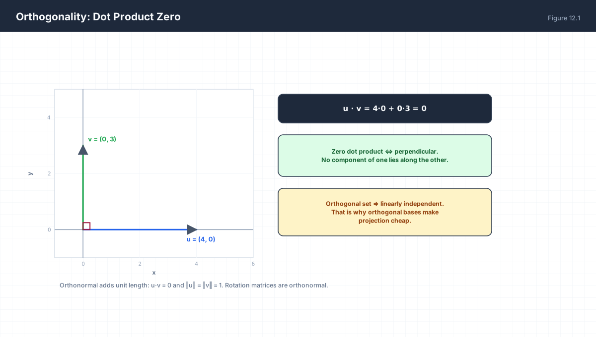
u ⊥ v   ⇔   u · v = 0

Orthonormal:  u·v = 0   and   ‖u‖ = ‖v‖ = 1
For an orthonormal matrix Q:  QᵀQ = I  ⇒  Q⁻¹ = Qᵀ
Orthogonal vectors are automatically linearly independent — if a combination Σcᵢqᵢ = 0, dotting with qⱼ isolates cⱼ‖qⱼ‖² = 0, so every coefficient is zero. That is why orthogonal bases make coordinate extraction trivial: you project instead of solving.
import numpy as np

u = np.array([1.0, 0.0, 0.0])
v = np.array([0.0, 3.0, 0.0])
print("u . v =", u @ v)                       # 0.0

Q = np.array([[0.0, -1.0], [1.0, 0.0]])       # 90-degree rotation
print("Q.T @ Q =\n", Q.T @ Q)
assert np.allclose(Q.T @ Q, np.eye(2))
print("inverse is the transpose:", np.allclose(np.linalg.inv(Q), Q.T))
3. Projection Onto a Vector
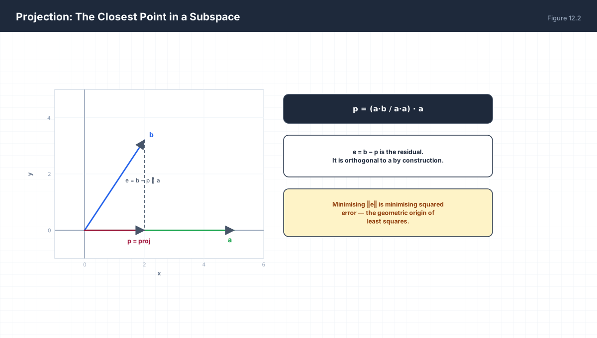
The projection of b onto a is the point on the line through a that is closest to b. “Closest” means the residual e = b − p is perpendicular to a — that condition defines the projection and yields the formula.
p = t·a                 p must lie on the line through a
e = b − p               the residual
e · a = 0               perpendicularity condition

(b − t·a) · a = 0
b·a − t(a·a) = 0
t = (a·b) / (a·a)

p = [(a·b) / (a·a)] · a
import numpy as np

a = np.array([5.0, 0.0])
b = np.array([2.0, 3.0])

t = (a @ b) / (a @ a)
p = t * a
e = b - p
print("t      :", t)                  # 0.4
print("p      :", p)                  # [2. 0.]
print("e      :", e)                  # [0. 3.]
print("e . a  :", e @ a)              # 0.0  -> orthogonal
assert np.isclose(e @ a, 0.0)
4. Least Squares
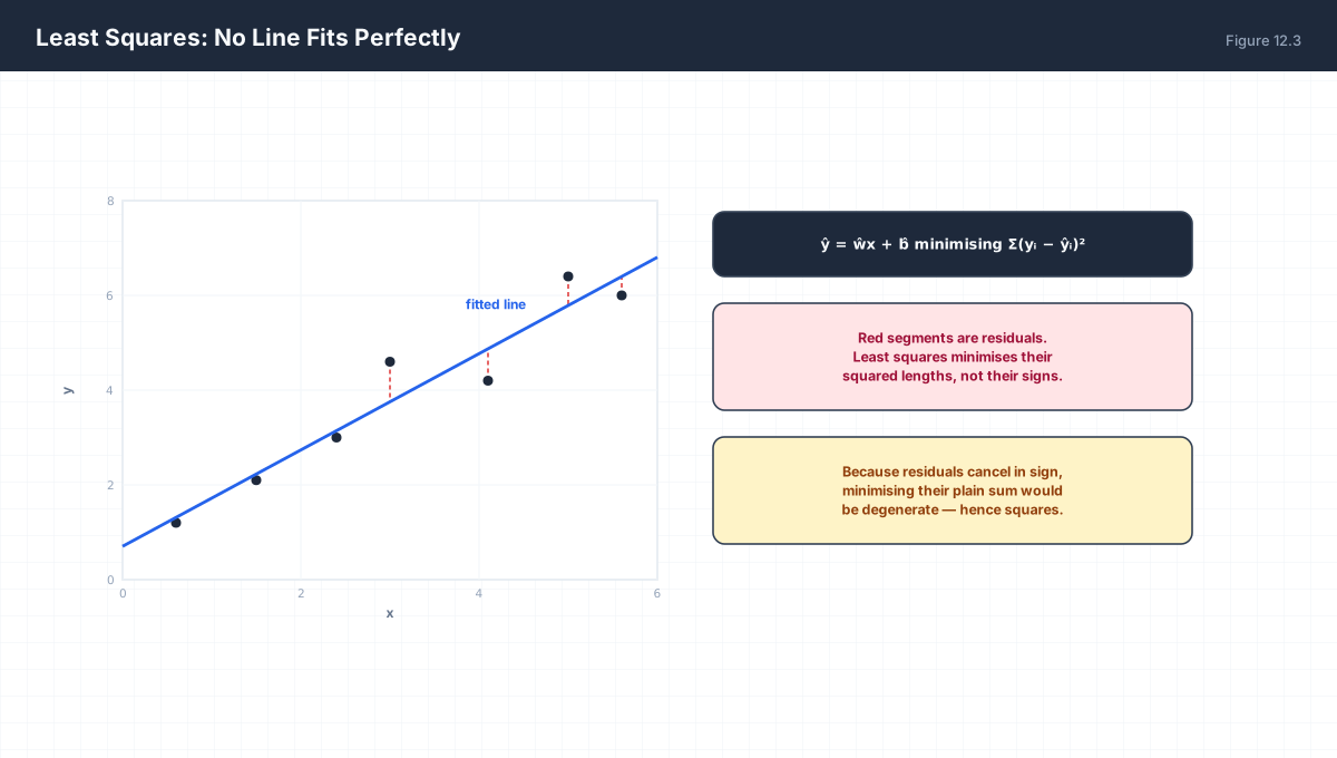
With more equations than unknowns the system is inconsistent: y is not in the column space of X, so there is no exact w. Instead you choose the ŵ whose prediction Xŵ is the projection of y onto that column space.
import numpy as np

rng = np.random.default_rng(7)
x = np.linspace(0, 5, 12)
y = 1.8 * x + 0.9 + rng.normal(0, 0.6, size=x.size)

X = np.column_stack([x, np.ones_like(x)])       # design matrix with intercept column
w, *_ = np.linalg.lstsq(X, y, rcond=None)
print("lstsq slope, intercept:", np.round(w, 4))

# compare against the closed form
w_closed = np.linalg.solve(X.T @ X, X.T @ y)
print("normal-eq solution     :", np.round(w_closed, 4))
assert np.allclose(w, w_closed, atol=1e-9)

pred = X @ w
resid = y - pred
print("residual is orthogonal to every column:")
print("  X0 . e =", round(X[:, 0] @ resid, 10))
print("  X1 . e =", round(X[:, 1] @ resid, 10))
The orthogonality prints are the real content. Least squares is not “the line that looks right” — it is the unique line whose residual vector is perpendicular to the design matrix’s column space. Everything else follows.
5. The Normal Equations
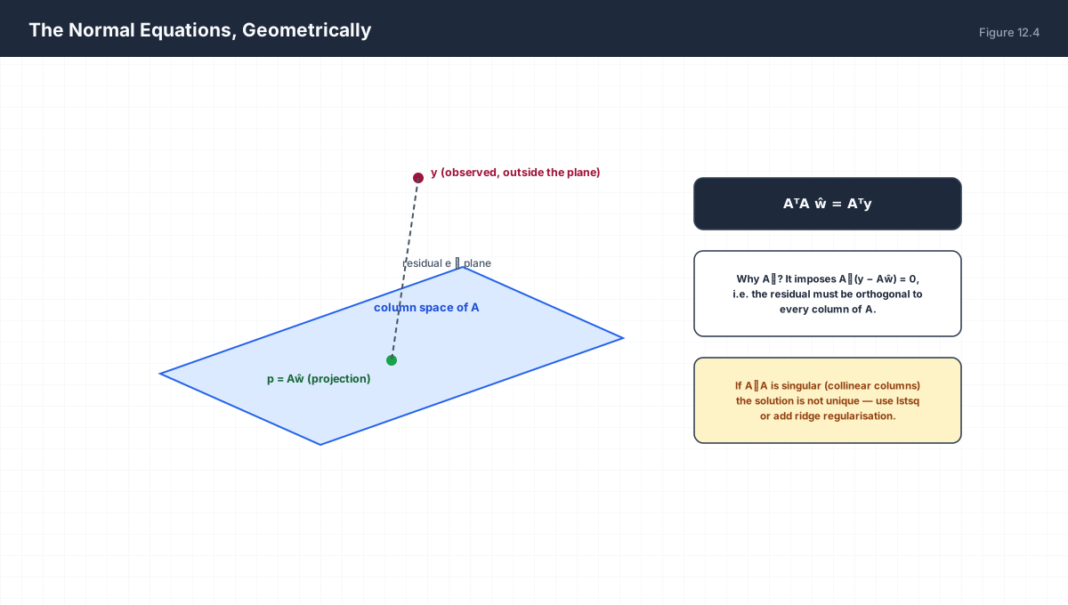
Require  Xᵀ(y − Xŵ) = 0        residual orthogonal to every column
⇒        Xᵀy − XᵀXŵ = 0
⇒        XᵀX ŵ = Xᵀy            the normal equations

If XᵀX is invertible:  ŵ = (XᵀX)⁻¹Xᵀy
| Situation | What Happens | Remedy |
|---|---|---|
Full rank X |
Unique solution exists | Use QR or lstsq |
| Collinear columns | XᵀX singular, infinite solutions |
Drop a column, or add ridge λI |
| Nearly collinear | κ(XᵀX) = κ(X)² — precision halves |
QR avoids squaring the condition number |
import numpy as np

# duplicated feature column -> singular XtX
X = np.array([[1.0, 1.0, 1.0],
              [2.0, 2.0, 1.0],
              [3.0, 3.0, 1.0]])
y = np.array([1.0, 2.0, 3.5])

print("rank X   :", np.linalg.matrix_rank(X))          # 2 of 3 columns
print("det XtX  :", round(np.linalg.det(X.T @ X), 12)) # 0.0

w, *_ = np.linalg.lstsq(X, y, rcond=None)              # still works
print("min-norm w:", np.round(w, 4))
print("first two weights are identical:", np.isclose(w[0], w[1]))
6. Gram–Schmidt and QR
import numpy as np

def gram_schmidt(V):
    """Return an orthonormal basis for the columns of V."""
    Q = []
    for v in V.T:
        w = v.astype(float).copy()
        for q in Q:
            w = w - (q @ w) * q
        norm = np.linalg.norm(w)
        if norm < 1e-12:
            raise ValueError("columns are linearly dependent")
        Q.append(w / norm)
    return np.column_stack(Q)

V = np.array([[1.0, 1.0, 0.0],
              [1.0, 0.0, 1.0],
              [0.0, 1.0, 1.0]])
Q = gram_schmidt(V)
print("Q:\n", np.round(Q, 4))
print("QᵀQ ≈ I:", np.allclose(Q.T @ Q, np.eye(Q.shape[1])))
assert np.allclose(Q.T @ Q, np.eye(Q.shape[1]))
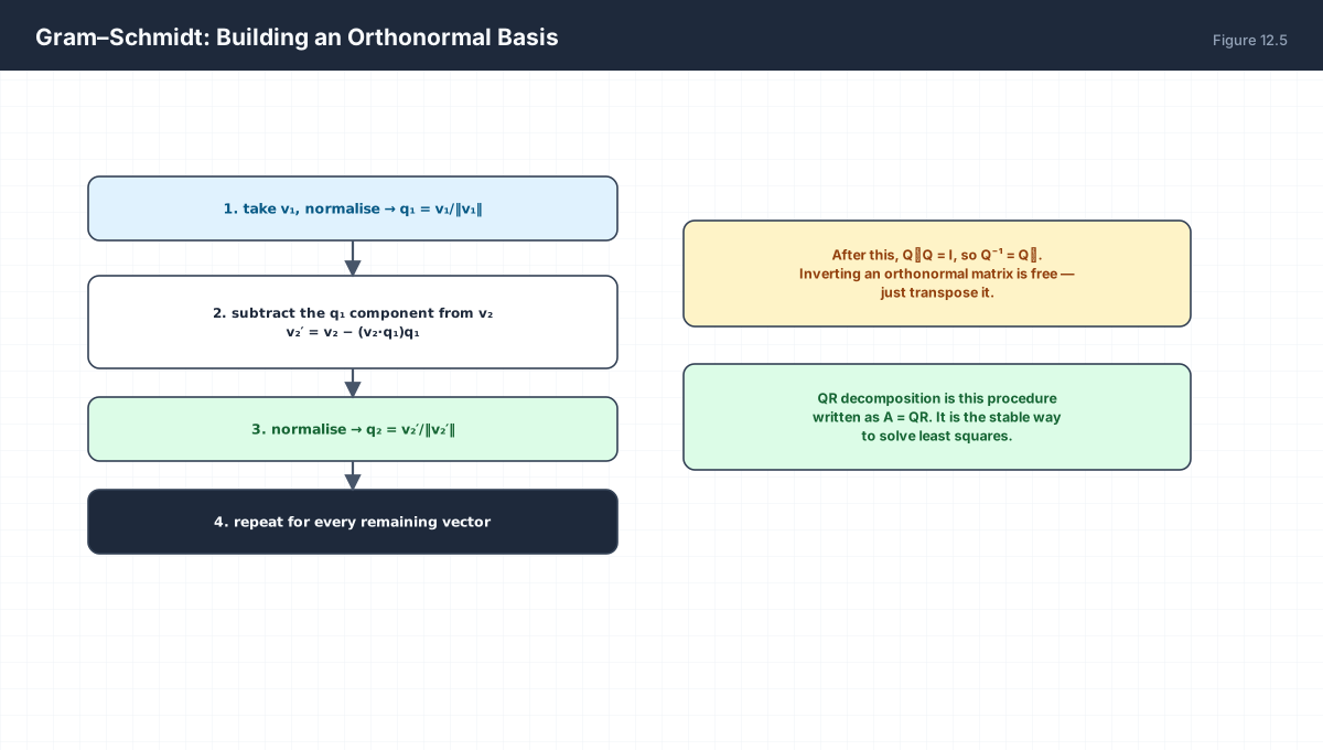
Gram–Schmidt as written is numerically fragile: repeated subtraction accumulates error when the inputs are nearly parallel. Production code uses Householder reflections (np.linalg.qr), which produce the same Q without that instability. The reason to care is that least squares via QR never forms XᵀX, so it never squares the condition number.
7. Worked Examples
7.1 Projection and residual
project (3,4) onto (1,0):
t = 3/1 = 3,  p = (3,0),  e = (0,4),  e·a = 0 ✓
7.2 Orthonormalise two vectors
v₁ = (3,4)  →  q₁ = (0.6, 0.8)
v₂ = (1,0)  →  v₂ − (v₂·q₁)q₁ = (1,0) − 0.6(0.6,0.8) = (0.64, −0.48)
               normalise → (0.8, −0.6)
q₁·q₂ = 0.48 − 0.48 = 0 ✓   both unit length ✓
7.3 Fit a line through three points
points (0,1), (1,2), (2,4)
design X = [[0,1],[1,1],[2,1]],  y = [1,2,4]
XᵀX = [[5,3],[3,3]],  Xᵀy = [10,7]
ŵ = (XᵀX)⁻¹ Xᵀy ≈ (1.5, 0.833)
line: ŷ = 1.5x + 0.833
7.4 Why not invert
If κ(X) = 10³, then κ(XᵀX) = 10⁶.
Double precision has ~16 digits, so ~10 survive — an order of
magnitude of accuracy lost purely from how you chose to compute.
7.5 Ridge as conditioning
(XᵀX + λI) ŵ = Xᵀy
Adding λI makes every eigenvalue at least λ, so the matrix is
always invertible. That is Ridge regression, and its purpose is
partly numeric, not only statistical.
8. Verify It in Python
import numpy as np

# --- 1. orthogonality and free inverse ----------------------------
Q = np.array([[0.0, -1.0], [1.0, 0.0]])
assert np.allclose(Q.T @ Q, np.eye(2))
assert np.allclose(np.linalg.inv(Q), Q.T)
print("orthogonal matrix: Q^-1 == Q.T")

# --- 2. projection formula and residual ---------------------------
a, b = np.array([5., 0.]), np.array([2., 3.])
p = ((a @ b) / (a @ a)) * a
assert np.allclose(p, [2., 0.])
assert np.isclose((b - p) @ a, 0.0)
print("projection:", p, " residual orthogonal")

# --- 3. projection is the closest point on the line ---------------
grid = np.linspace(-5, 10, 4001)
pts = np.array([[t * a[0], t * a[1]] for t in grid])
dists = np.linalg.norm(pts - b, axis=1)
closest = pts[np.argmin(dists)]
assert np.allclose(closest, p, atol=1e-2)
print("projection minimises distance: ", np.round(closest, 3))

# --- 4. normal equations agree with lstsq -------------------------
rng = np.random.default_rng(3)
x = np.linspace(0, 4, 10)
y = 2.5 * x - 1.0 + rng.normal(0, 0.3, x.size)
X = np.column_stack([x, np.ones_like(x)])

w_ls, *_ = np.linalg.lstsq(X, y, rcond=None)
w_ne = np.linalg.solve(X.T @ X, X.T @ y)
assert np.allclose(w_ls, w_ne, atol=1e-9)
print("lstsq == normal equations:", np.round(w_ls, 4))

# --- 5. residual orthogonal to column space -----------------------
e = y - X @ w_ls
assert np.allclose(X.T @ e, 0.0, atol=1e-9)
print("X^T e ~ 0:", np.round(X.T @ e, 12))

# --- 6. QR beats normal equations on a bad matrix -----------------
bad = np.array([[1.0, 1.0], [1.0, 1.0 + 1e-8]])
print("kappa(X)   :", f"{np.linalg.cond(bad):.3e}")
print("kappa(XtX) :", f"{np.linalg.cond(bad.T @ bad):.3e}")
assert np.linalg.cond(bad.T @ bad) > 1e10
Qm, Rm = np.linalg.qr(bad)
assert np.allclose(Qm @ Rm, bad)
print("QR reconstruction exact")

# --- 7. Gram-Schmidt yields an orthonormal basis ------------------
def gs(V):
    out = []
    for v in V.T:
        w = v.astype(float).copy()
        for q in out:
            w -= (q @ w) * q
        out.append(w / np.linalg.norm(w))
    return np.column_stack(out)

V = np.array([[1., 1., 0.], [1., 0., 1.], [0., 1., 1.]])
G = gs(V)
assert np.allclose(G.T @ G, np.eye(3))
print("Gram-Schmidt orthonormal:", np.allclose(G.T @ G, np.eye(3)))

# --- 8. ridge makes an otherwise singular system solvable ---------
lam = 1e-3
rhs = bad.T @ np.array([1.0, 2.0])
w_ridge = np.linalg.solve(bad.T @ bad + lam * np.eye(2), rhs)
assert np.all(np.isfinite(w_ridge))
print("ridge solution:", np.round(w_ridge, 4))
print("all assertions passed")
9. Practice Questions
- Test
(1,2,2)and(2,−2,1)for orthogonality. - Project
(3,4)onto(1,0); give p and e and verify e ⊥ a. - Project
(1,1)onto the line spanned by(1,1)— what happens and why? - Derive
t = (a·b)/(a·a)from the orthogonality condition. - Write the normal equations and state the invertibility condition.
- What is
κ(XᵀX)in terms ofκ(X), and why does it matter? - Show that
Xᵀe = 0at the least-squares solution. - Orthonormalise
(1,0,0)and(1,1,0). - Why does ridge regularisation make the system solvable?
- Why is QR preferred over the normal equations for least squares?
10. Official References & Further Reading
Continue the Course
- Course Index: AI Mathematics Masterclass — All 48 Chapters
- Previous Chapter: Chapter 11: Norms, Distances & Similarity Measures
- Next Chapter: Chapter 13: Eigenvalues, Eigenvectors & Diagonalization
- Related Series: PyTorch Engineering Masterclass — All 16 Modules