
AI Reading
Quick summary of this article
AI Mathematics Masterclass — Chapter 6 of 48
Training a neural network is the repeated application of one question: if I nudge this parameter slightly, how much does the loss change? That question is the derivative, and the derivative is defined as a limit. This chapter builds the limit honestly, shows where continuity breaks, derives the derivative from the difference quotient, and then demonstrates the numerical trap that catches every practitioner: the step size that gives the worst numerical derivative sits between the two errors you were trying to trade off.
1. Technical Audit & Core Learning Objectives
Calculus is often introduced as a bag of differentiation rules to be memorised, with limits skipped as “formalities”. The rules are the easy part. The hard parts are knowing when a derivative does not exist, and knowing why finite differences are not a substitute for autodiff.
| Component | Common Tutorial Deficiency | Engineering Standard Applied Here |
|---|---|---|
| Limits | Dismissed as a formality, so the definition of the derivative feels arbitrary. | Built first, then used to derive the derivative rather than assert it. |
| Continuity | Conflated with differentiability; the ReLU corner never explained. | The three discontinuity types drawn, then ReLU located precisely in that taxonomy. |
| Rules | Power, product, quotient listed without derivation or use. | Each derived from the limit definition and immediately exercised on a loss function. |
| Numerics | Never mentioned; students compute finite differences and trust them. | Truncation vs round-off measured, the sweet spot located empirically. |
Core learning objectives. After this chapter you should be able to:
- Evaluate one-sided and two-sided limits and state when a limit fails to exist.
- Classify a discontinuity as removable, jump, or infinite.
- Derive the derivative of
x²from the difference quotient. - Apply the power, constant-multiple, sum, product, quotient, and chain rules.
- Interpret the sign and magnitude of
f′geometrically and in optimiser terms. - Explain the truncation/round-off trade-off and why autodiff avoids both.
2. Limits: What Happens as We Approach
The limit lim_{x→a} f(x) = L says: as x gets arbitrarily close to a (without necessarily equalling it), f(x) gets arbitrarily close to L. The value of f(a) itself is irrelevant — the limit describes the approach, not the arrival.
lim_{x→2} (x² − 4)/(x − 2)

Direct substitution gives 0/0 -- indeterminate, not an answer.
Factor:  (x−2)(x+2)/(x−2) = x + 2   for x ≠ 2
Limit:   lim = 4

The function is undefined at x = 2 but has a perfectly good limit there.
That gap between "undefined at" and "limit at" is the removable discontinuity.
| Case | Meaning | Example |
|---|---|---|
| Two-sided exists | Left limit = right limit | lim x² at any point |
| One-sided only | Sides disagree | |x|/x at 0: −1 vs +1 |
| Infinite | Grows without bound | 1/x as x→0⁺ |
3. Continuity and Its Three Failure Modes
A function is continuous at a when three things hold: f(a) is defined, the limit exists, and the two are equal. Each failure gives a distinct kind of break.
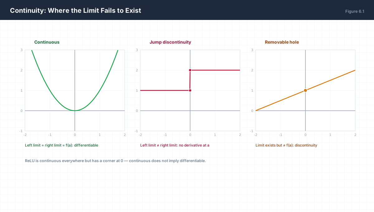
| Type | Diagnosis | In Practice |
|---|---|---|
| Removable | Limit exists, f(a) differs or is undefined |
A hole; fixable by redefining f(a) |
| Jump | One-sided limits differ | Step functions, hard quantisation, sign() |
| Infinite | Limit is unbounded | Vertical asymptote, log(0), division by zero |
Continuity does not imply differentiability. ReLU is continuous at zero but has a corner there, and the derivative does not exist at a corner. This is why frameworks use a subgradient convention at exactly 0 rather than claiming a derivative exists. The convention is arbitrary and harmless: the probability of a float landing exactly on zero is negligible, and any value in [0, 1] gives the same first-order behaviour.
4. The Derivative as the Limit of a Secant Slope
Pick two points on a curve and the slope between them is the average rate of change. Slide them together until the gap vanishes and the average becomes instantaneous.
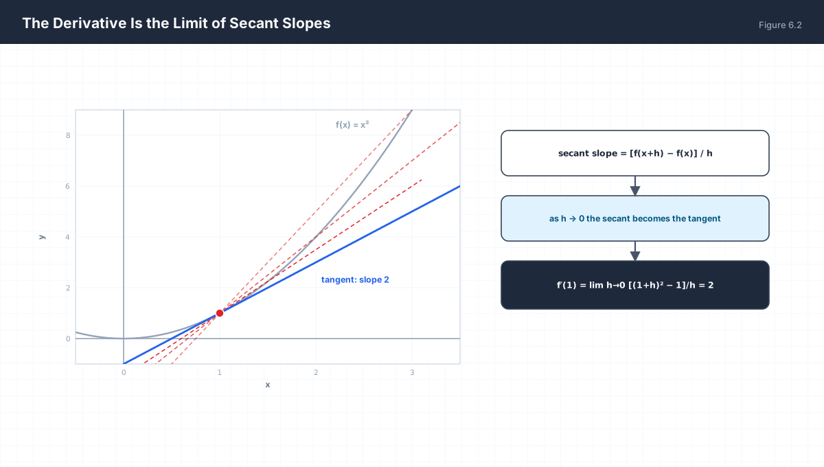
h, converging to the tangent. The derivative is the limit of that family.f′(x) = lim_{h→0} [f(x + h) − f(x)] / h
For f(x) = x²:
[ (x+h)² − x² ] / h
= [ x² + 2xh + h² − x² ] / h
= [ 2xh + h² ] / h
= 2x + h (valid for h ≠ 0)
As h → 0: f′(x) = 2x
Note the structure: the h in the denominator cancels the h that appears in the numerator. That cancellation is what makes the limit exist. If it does not cancel, the function is not differentiable there — which is exactly what happens at |x| at zero, where the left quotient gives −1 and the right gives +1.
5. Reading the Derivative
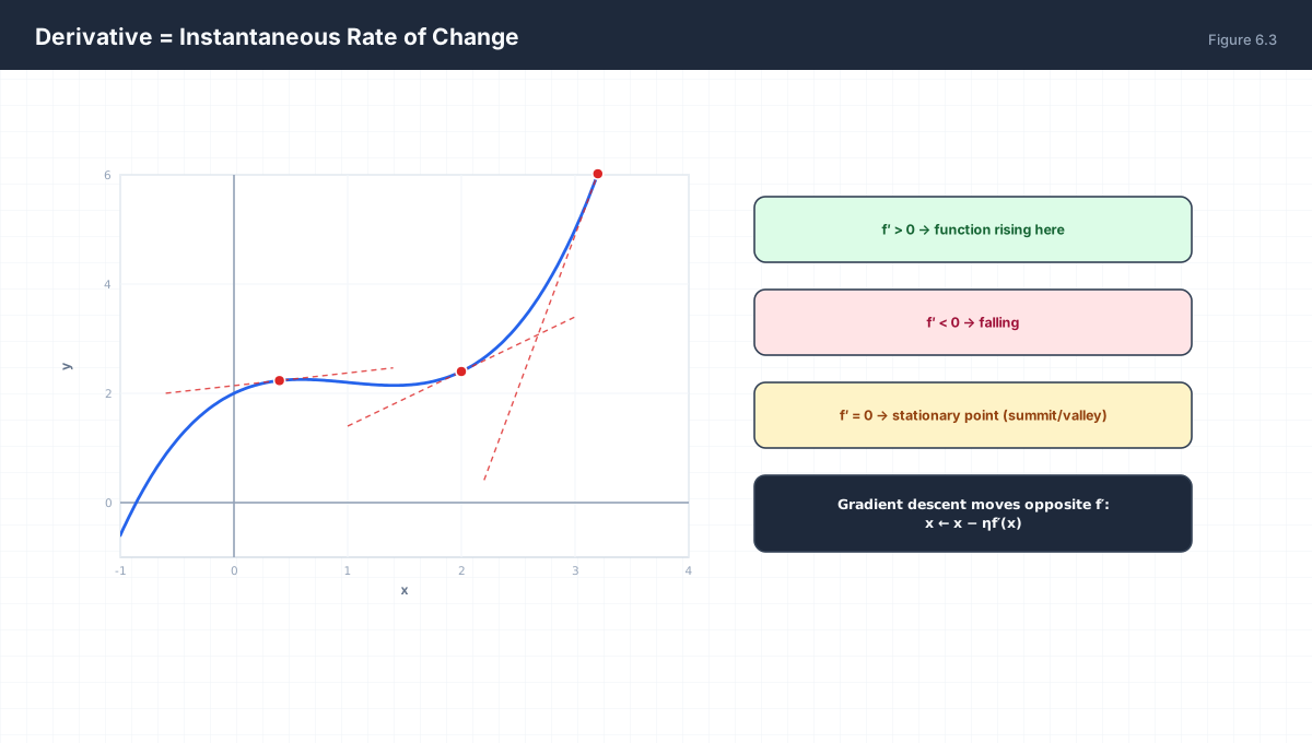
f′ tells you the direction of travel; the magnitude tells you how fast.| Sign / Value | Geometry | Optimiser Meaning |
|---|---|---|
f′ > 0 |
Rising | Decrease the parameter to reduce loss |
f′ < 0 |
Falling | Increase the parameter |
f′ = 0 |
Flat | Stationary: minimum, maximum, or saddle |
|f′| large |
Steep | Large step unless the learning rate is small |
5.1 The rules, all derived from the definition
power        d/dx xⁿ     = n·xⁿ⁻¹
constant     d/dx c      = 0
multiple     d/dx c·f    = c·f′
sum          d/dx (f+g)  = f′ + g′
product      d/dx f·g    = f′g + fg′
quotient     d/dx f/g    = (f′g − fg′) / g²
chain        d/dx f(g(x)) = f′(g(x)) · g′(x)
The chain rule is the one that matters for deep learning; Chapter 21 is devoted to it. The others are best memorised and then sanity-checked against a small numerical example.
6. Numerical Differentiation and Its Trap
Replacing the limit with a small finite h gives a computable approximation. It also introduces two competing errors.
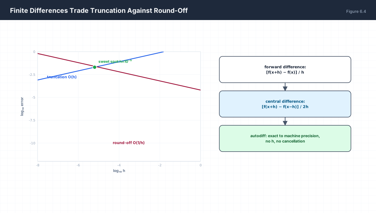
h shrinks; round-off rises. The best step size is where they cross, not as small as possible.import numpy as np
def forward_diff(f, x, h=1e-5):
return (f(x + h) - f(x)) / h
def central_diff(f, x, h=1e-5):
return (f(x + h) - f(x - h)) / (2 * h)
f = lambda t: t ** 3
exact = lambda t: 3 * t ** 2
x0 = 1.5
print("exact :", exact(x0)) # 6.75
print("forward :", forward_diff(f, x0))
print("central :", central_diff(f, x0))
# shrink h and watch the error turn around
for h in (1e-2, 1e-5, 1e-8, 1e-12, 1e-15):
err = abs(central_diff(f, x0, h) - exact(x0))
print(f"h={h:.0e} abs error={err:.3e}")
The turnaround is the whole lesson. Shrinking h reduces truncation error — the error from not actually reaching the limit, which scales like h² for the central formula. But it increases round-off error, because f(x+h) − f(x) becomes the difference of two nearly equal floats and catastrophic cancellation destroys the significant digits. At h ≈ 10⁻⁵ for float64 the errors cross, and below that accuracy collapses. Central differences are also second-order accurate versus first-order for forward differences, which is why they are preferred when a gradient must be estimated.
None of this is a problem in practice, because autodiff does not approximate anything — it propagates exact derivatives through the computation graph using the chain rule. Finite differences survive mainly as a debugging check: if an analytic gradient disagrees with the central difference, the analytic gradient has a bug.
7. From Derivative to Descent
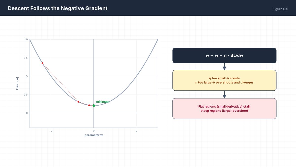
w ← w − η · dL/dw

If dL/dw > 0, w decreases, so L decreases.     (moving against the gradient)
If dL/dw < 0, w increases, so L decreases.     (same rule, opposite sign)
At dL/dw = 0, nothing moves.                   (a stationary point)

The update is a first-order Taylor argument:
  L(w − ηg) ≈ L(w) − ηg²  ≤  L(w)      for small enough η
Two failure modes are visible directly in the figure. If η is too large the step overshoots the minimum and the next gradient points back, producing oscillation or divergence. If the surface is flat the gradient vanishes and progress stalls — the same mechanism as the saturated sigmoid in Chapter 3, now seen from the optimiser's side.
import numpy as np

L    = lambda w: (w - 3.0) ** 2 + 1.0      # minimum at w = 3
grad = lambda w: 2.0 * (w - 3.0)

for eta in (0.05, 0.9, 1.05):
    w, path = 0.0, [0.0]
    for _ in range(12):
        w = w - eta * grad(w)
        path.append(round(w, 4))
    print(f"eta={eta:<5} final w={w:8.4f}  loss={L(w):8.4f}")
With η = 0.05 the iterates crawl toward 3. With η = 0.9 they converge quickly. With η = 1.05 the step is larger than the curvature allows, so each iteration overshoots by more than it corrects and the sequence diverges — the discrete analogue of an unstable differential equation.
8. Worked Examples
8.1 Evaluate a limit by factoring
lim_{x→3} (x² − 9)/(x − 3)
= lim (x−3)(x+3)/(x−3)
= lim (x + 3) = 6
8.2 Show a limit does not exist
f(x) = |x| / x
left  limit (x→0⁻): −1
right limit (x→0⁺): +1
Sides disagree → the two-sided limit does not exist.
8.3 Differentiate a loss by the rules
For L(w) = (w − y)² with y constant, find dL/dw.
Let u = w − y,  so L = u²
dL/du = 2u          (power rule)
du/dw = 1           (sum rule, y constant)
dL/dw = 2u · 1 = 2(w − y)    (chain rule)
8.4 Product rule on a regulariser
Differentiate f(w) = w²·ln(w) for w > 0.
f′ = (2w)(ln w) + (w²)(1/w) = 2w·ln w + w
8.5 Estimate the derivative numerically and compare
f(x) = x³ at x = 1.5, exact f′ = 3(1.5)² = 6.75

forward, h = 1e-5:   (1.50001³ − 1.5³)/1e-5  ≈ 6.7500450   error ~4.5e-5
central, h = 1e-5:   ≈ 6.750000000            error ~1e-10
9. Verify It in Python
import numpy as np

# --- 1. A removable discontinuity has a limit ----------------------
g = lambda x: (x ** 2 - 4) / (x - 2)
xs = np.array([1.999999, 2.000001])
print("approach 4 from both sides:", np.round(g(xs), 6))
assert np.allclose(g(xs), 4, atol=1e-4)

# --- 2. |x|/x has no two-sided limit -------------------------------
h = lambda x: abs(x) / x
assert h(-1e-9) == -1.0 and h(1e-9) == 1.0
print("left/right limits disagree:", h(-1e-9), h(1e-9))

# --- 3. Derivative of x^2 from the difference quotient ------------
f = lambda x: x * x
for hh in (1e-1, 1e-3, 1e-6):
    est = (f(3 + hh) - f(3)) / hh
    print(f"h={hh:.0e}  quotient={est:.9f}  (exact 6)")

# --- 4. Central difference is second-order accurate ---------------
exact = 3 * 1.5 ** 2
c = lambda t: t ** 3
errs = {}
for hh in (1e-2, 1e-4, 1e-6):
    est = (c(1.5 + hh) - c(1.5 - hh)) / (2 * hh)
    errs[hh] = abs(est - exact)
assert errs[1e-6] < errs[1e-2] * 1e-4        # shrinking h^2 shrinks error fast
print("central-diff errors:", {f"{k:.0e}": f"{v:.2e}" for k, v in errs.items()})

# --- 5. Round-off eventually dominates ----------------------------
tiny = abs((c(1.5 + 1e-15) - c(1.5 - 1e-15)) / (2e-15) - exact)
assert tiny > errs[1e-6]                     # worse than a much larger h
print("error at h=1e-15 is worse:", f"{tiny:.2e}")

# --- 6. Descent converges or diverges by learning rate ------------
L2 = lambda w: (w - 3.0) ** 2 + 1.0
gr = lambda w: 2.0 * (w - 3.0)

def run(eta, steps=40):
    w = 0.0
    for _ in range(steps):
        w -= eta * gr(w)
    return w

assert abs(run(0.9) - 3.0) < 1e-3            # converges
assert abs(run(1.05)) > 100                  # diverges
print("eta=0.9 ->", round(run(0.9), 4), " eta=1.05 ->", round(run(1.05), 1))
print("all assertions passed")
10. Practice Questions
- Evaluate
lim_{x→2} (x² − 4)/(x − 2)and name the discontinuity type of the original function at 2. - Show that
|x|/xhas no two-sided limit at 0, then state its one-sided limits. - State the three conditions required for continuity at a point.
- Derive
d/dx x³from the limit definition. - Differentiate
f(x) = 3x⁴ − 2x + 7and evaluate atx = 1. - Apply the product rule to
x·eˣ. - Apply the quotient rule to
(x+1)/(x−1). - Why is ReLU continuous but not differentiable at zero, and what convention do frameworks use?
- Explain in one sentence why a smaller
heventually makes a numerical derivative worse. - For
L(w) = (w−3)²+1, compute the gradient atw = 0and state which direction the update moves.
11. Official References & Further Reading
Continue the Course
- Course Index: AI Mathematics Masterclass — All 48 Chapters
- Previous Chapter: Chapter 5: Summation Notation, Sequences & Series
- Next Chapter: Chapter 7: Scalars, Vectors & Vector Spaces
- Related Series: PyTorch Engineering Masterclass — All 16 Modules