
AI Reading
Quick summary of this article
AI Mathematics Masterclass — Chapter 14 of 48
The singular value decomposition is the most useful factorization in applied linear algebra, and the one most machine-learning practitioners use without knowing it. PCA is an SVD. LoRA is a low-rank SVD-shaped constraint. Every condition number is a ratio of singular values. This chapter builds the decomposition geometrically — rotate, scale, rotate — explains what singular values rank, derives the best low-rank approximation, and connects it to the eigendecomposition it generalises.
1. Technical Audit & Core Learning Objectives
| Component | Common Tutorial Deficiency | Engineering Standard Applied Here |
|---|---|---|
| Geometry | Formula A = UΣVᵀ given with no interpretation. |
Presented as rotate → scale → rotate, with the rectangular case explained. |
| Singular values | Treated as unexplained scalars. | Framed as an importance ranking over directions. |
| Truncation | Compression shown without the optimality guarantee. | Eckart–Young stated and verified numerically. |
| Relationship to eigen | Never connected, leaving two disjoint tools. | SVD derived from AᵀA and AAᵀ, with the numerical caveat. |
Core learning objectives. After this chapter you should be able to:
- State the shapes of
U,Σ, andVᵀfor a rectangular matrix. - Interpret
UandVas orthonormal bases andΣas an importance ranking. - Construct a rank-
kapproximation and state why it is optimal. - Relate singular values to eigenvalues of
AᵀA. - Compute a condition number from singular values.
- Identify PCA, LoRA, and the pseudo-inverse as SVD applications.
2. Rotate, Scale, Rotate
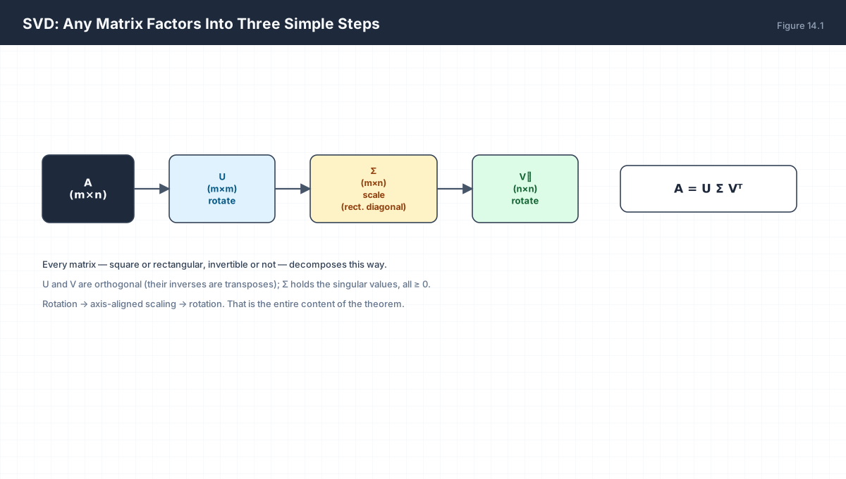
A = U Σ Vᵀ                 A is (m×n)

U   (m×m)  orthogonal     left singular vectors   — rotate output
Σ   (m×n)  diagonal       singular values σᵢ ≥ 0  — scale axes
Vᵀ  (n×n)  orthogonal     right singular vectors  — rotate input

Compare with eigendecomposition, which requires a square matrix
and a diagonalizable one. SVD exists for every matrix, always.
import numpy as np

A = np.array([[3.0, 1.0],
              [1.0, 3.0],
              [0.0, 2.0]])          # 3x2, not square
U, s, Vt = np.linalg.svd(A, full_matrices=False)

print("U :", U.shape)              # (3, 2)
print("s :", np.round(s, 4))       # singular values, descending
print("Vt:", Vt.shape)             # (2, 2)

# reconstruct: Sigma is rectangular, so build it explicitly
Sigma = np.zeros((U.shape[1], Vt.shape[0]))
np.fill_diagonal(Sigma, s)
print("reconstruction exact:", np.allclose(U @ Sigma @ Vt, A))
print("U orthonormal:", np.allclose(U.T @ U, np.eye(2)))
print("V orthonormal:", np.allclose(Vt @ Vt.T, np.eye(2)))
Note full_matrices=False. With it, U is (m×k) and Vt is (k×n) where k = min(m,n), and the reconstruction needs a k×k diagonal middle term. With the default True you get full square U and Vt, and the extra columns multiply by zero singular values — correct but wasteful.
3. Singular Values Rank Directions
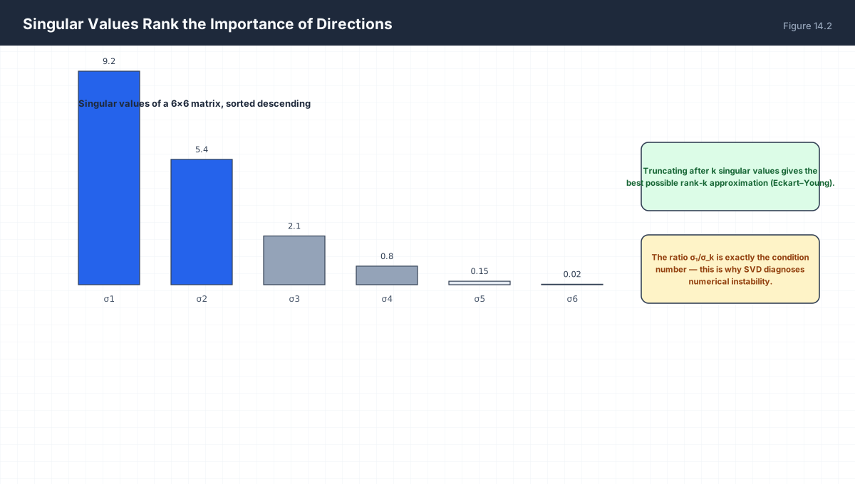
| Quantity | Definition | Meaning |
|---|---|---|
| σ₁ | Largest singular value | Maximum stretch of any unit vector |
| rank | Count of non-zero σ | Dimension of the image |
| κ | σ₁/σₙ |
Condition number, the error amplifier |
| ‖A‖₂ | σ₁ |
Spectral norm — used in spectral normalisation |
import numpy as np

rng = np.random.default_rng(0)
A = rng.normal(size=(6, 6))
s = np.linalg.svd(A, compute_uv=False)
print("singular values:", np.round(s, 3))
print("condition number:", round(s[0] / s[-1], 2))
assert np.isclose(np.linalg.norm(A, 2), s[0])          # spectral norm is s[0]
print("spectral norm == s[0]:", np.isclose(np.linalg.norm(A, 2), s[0]))

# a deliberately rank-deficient matrix
B = np.outer(np.arange(1., 6.), np.arange(1., 6.))
sb = np.linalg.svd(B, compute_uv=False)
print("rank-deficient spectrum:", np.round(sb, 10))     # only one non-zero
4. Low-Rank Approximation
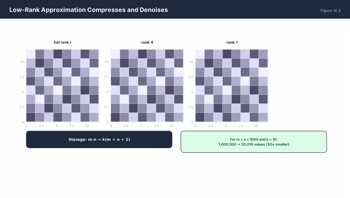
Aₖ = Σᵢ₌₁ᵏ σᵢ uᵢ vᵢᵀ

Eckart–Young theorem: among all matrices of rank ≤ k,
Aₖ minimises ‖A − B‖ for both the spectral and Frobenius norms.

Storage: m·n  →  k(m + n + 1)
import numpy as np

rng = np.random.default_rng(2)
A = rng.normal(size=(40, 30))
U, s, Vt = np.linalg.svd(A, full_matrices=False)

def rank_k(U, s, Vt, k):
    return (U[:, :k] * s[:k]) @ Vt[:k, :]

for k in (1, 5, 15, 30):
    err = np.linalg.norm(A - rank_k(U, s, Vt, k), "fro")
    print(f"k={k:3d}  Frobenius error = {err:.3f}")

# the error of truncation equals the discarded tail
assert np.isclose(np.linalg.norm(A - rank_k(U, s, Vt, 5), "fro"),
                  np.sqrt((s[5:] ** 2).sum()))
print("truncation error == norm of discarded singular values")
The last assertion is the useful identity: the Frobenius error of a rank-k truncation is exactly the L2 norm of the discarded singular values. You can therefore predict the compression error before deciding what to discard.
5. SVD and Eigendecomposition
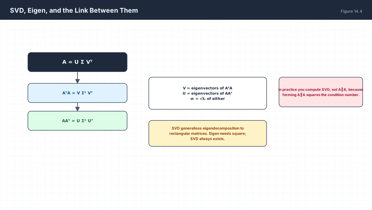
A  = U Σ Vᵀ
AᵀA = V Σ² Vᵀ        V = eigenvectors of AᵀA
AAᵀ = U Σ² Uᵀ        U = eigenvectors of AAᵀ
σᵢ = √λᵢ             singular values are square roots of those eigenvalues
import numpy as np

A = np.array([[2.0, 1.0, 0.0],
              [1.0, 2.0, 1.0]])
U, s, Vt = np.linalg.svd(A, full_matrices=False)

evals_AtA, evecs_AtA = np.linalg.eigh(A.T @ A)
evals_AtA = evals_AtA[::-1]                     # descending
evecs_AtA = evecs_AtA[:, ::-1]

k = s.size                                  # A is (2,3) so there are only 2 singular values
gram_sv = np.sqrt(np.clip(evals_AtA, 0, None))[:k]
print("sigma from svd      :", np.round(s, 6))
print("sqrt(eig of A^T A)  :", np.round(gram_sv, 6))
assert np.allclose(s, gram_sv)
print("V columns match eigenvectors (up to sign):",
      np.allclose(np.abs(Vt.T), np.abs(evecs_AtA[:, :k])))
The phrase “up to sign” matters. An eigenvector can be negated without changing anything, so comparing eigenvectors requires comparing absolute values or checking the subspace. This is why comparing two SVD outputs directly is unreliable even when both are correct.
6. Why You Use SVD Instead of Forming AᵀA
Mathematically, AᵀA is enough to get the singular values. Numerically, it is a trap:
import numpy as np

A = np.array([[1.0, 1.0], [1.0, 1.0 + 1e-8]])
print("kappa(A)    :", f"{np.linalg.cond(A):.3e}")
print("kappa(A^T A):", f"{np.linalg.cond(A.T @ A):.3e}")

s_svd = np.linalg.svd(A, compute_uv=False)
s_gram = np.sqrt(np.clip(np.linalg.eigvalsh(A.T @ A)[::-1], 0, None))
print("sigma via SVD  :", s_svd)
print("sigma via Gram :", s_gram)
print("relative difference:", np.abs(s_svd - s_gram).max() / s_svd[0])
Forming AᵀA squares the condition number, so κ(AᵀA) = κ(A)². In the example above that is a jump from 10⁸ to 10¹⁶, which is at the limit of double precision — the smallest singular values are no longer recoverable accurately. Always call np.linalg.svd on A; never diagonalize AᵀA unless you have a specific reason.
7. Where SVD Appears
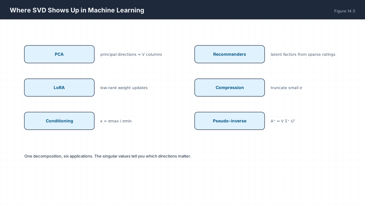
| Application | SVD Form | What Is Used |
|---|---|---|
| PCA | centred X = UΣVᵀ |
Columns of V are the principal directions |
| Pseudo-inverse | A⁺ = VΣ⁺Uᵀ |
Reciprocate non-zero σ, zero the rest |
| LoRA | ΔW = BA, rank r |
Assumes updates are low-rank |
| Spectral norm | σ₁ |
Bound on layer amplification |
| Recommenders | truncated SVD of ratings | Latent user and item factors |
8. Worked Examples
8.1 Shapes of a rectangular SVD
A is (5×3):
  U  (5×5) or (5×3) with full_matrices=False
  Σ  (5×3) — three non-zero diagonal entries at most
  Vᵀ (3×3)
  rank ≤ 3
8.2 Singular values of a scaled matrix
If B = cA, then σᵢ(B) = |c| σᵢ(A).
Scaling scales the spectrum linearly — and κ is unchanged.
8.3 Singular values of a rotation
Rotations preserve length, so every σᵢ = 1 and κ = 1.
A perfectly conditioned matrix.
8.4 Rank from the spectrum
A = [[1,2],[2,4]]:  σ = (√25, 0) ≈ (5, 0)
Exactly one non-zero singular value → rank 1.
8.5 Reconstruction error is the tail
σ = (9.2, 5.4, 2.1, 0.8)
k = 2 → ‖A − A₂‖_F = √(2.1² + 0.8²) = √(4.41+0.64) = 2.247
9. Verify It in Python
import numpy as np

# --- 1. reconstruction for a rectangular matrix -------------------
A = np.array([[3., 1.], [1., 3.], [0., 2.]])
U, s, Vt = np.linalg.svd(A, full_matrices=False)
Sigma = np.zeros((U.shape[1], Vt.shape[0]))
np.fill_diagonal(Sigma, s)
assert np.allclose(U @ Sigma @ Vt, A)
print("3x2 reconstruction exact, shapes:", U.shape, Sigma.shape, Vt.shape)

# --- 2. orthonormality --------------------------------------------
assert np.allclose(U.T @ U, np.eye(U.shape[1]))
assert np.allclose(Vt @ Vt.T, np.eye(Vt.shape[0]))
print("U and V orthonormal")

# --- 3. singular values are sorted and non-negative ---------------
rng = np.random.default_rng(0)
B = rng.normal(size=(8, 5))
sb = np.linalg.svd(B, compute_uv=False)
assert np.all(sb >= 0) and np.all(np.diff(sb) <= 1e-12)
print("sigma sorted descending:", np.round(sb, 3))

# --- 4. spectral norm is sigma_1 ----------------------------------
assert np.isclose(np.linalg.norm(B, 2), sb[0])
print("||B||_2 == sigma_1")

# --- 5. Eckart-Young: truncation error is the tail ---------------
Ub, sbu, Vtb = np.linalg.svd(B, full_matrices=False)
for k in (1, 3, 5):
    Ak = (Ub[:, :k] * sbu[:k]) @ Vtb[:k, :]
    err = np.linalg.norm(B - Ak, "fro")
    tail = np.sqrt((sbu[k:] ** 2).sum())
    assert np.isclose(err, tail)
print("truncation error == discarded tail for every k")

# --- 6. rank counts non-zero singular values ---------------------
deficient = np.outer(np.arange(1., 6.), np.arange(1., 6.))
sd = np.linalg.svd(deficient, compute_uv=False)
assert np.sum(sd > 1e-10) == 1 == np.linalg.matrix_rank(deficient)
print("rank from spectrum:", np.sum(sd > 1e-10))

# --- 7. sigma are sqrt of A^T A eigenvalues ----------------------
ev = np.linalg.eigvalsh(B.T @ B)[::-1]
assert np.allclose(sb, np.sqrt(np.clip(ev, 0, None)))
print("sigma == sqrt(eig(A^T A))")

# --- 8. condition number from the spectrum -----------------------
cond = sb[0] / sb[-1]
assert np.isclose(cond, np.linalg.cond(B))
print("kappa from sigma:", round(cond, 3))

# --- 9. forming A^T A squares the conditioning -------------------
bad = np.array([[1., 1.], [1., 1. + 1e-8]])
assert np.linalg.cond(bad.T @ bad) > 1e10
print("kappa(A):", f"{np.linalg.cond(bad):.2e}",
      " kappa(A^T A):", f"{np.linalg.cond(bad.T @ bad):.2e}")
print("all assertions passed")
10. Practice Questions
- State the shapes of
U,Σ,Vᵀfor a(4×6)matrix withfull_matrices=False. - Why is
Σrectangular, and where do the singular values sit in it? - Prove that
σᵢ(cA) = |c|σᵢ(A). - What are the singular values of an orthogonal matrix, and its condition number?
- State the Eckart–Young theorem and one practical use.
- Express the Frobenius truncation error in terms of discarded
σ. - Derive
AᵀA = VΣ²VᵀfromA = UΣVᵀ. - Why is diagonalizing
AᵀAnumerically worse than callingsvd(A)? - How many values does a rank-
kapproximation store for an(m×n)matrix? - Explain PCA using only SVD vocabulary.
11. Official References & Further Reading
Continue the Course
- Course Index: AI Mathematics Masterclass — All 48 Chapters
- Previous Chapter: Chapter 13: Eigenvalues, Eigenvectors & Diagonalization
- Next Chapter: Chapter 15: Rank, Null Space & Solvability of Linear Systems
- Related Series: PyTorch Engineering Masterclass — All 16 Modules