
AI Reading
Quick summary of this article
AI Mathematics Masterclass — Chapter 18 of 48
Everything in this part of the course now has a place in a transformer. A linear layer is one matrix product plus a broadcast add. Attention is three of those, a contraction, and a softmax. Layer normalisation is a row-wise rescaling by two statistics. Backpropagation is two more matrix products, one of them transposed. This chapter assembles the pieces and shows that a modern architecture contains exactly seven distinct linear-algebraic operations, repeated at scale.
1. Technical Audit & Core Learning Objectives
| Component | Common Tutorial Deficiency | Engineering Standard Applied Here |
|---|---|---|
| Linear layer | Treated as an opaque nn.Linear call. |
Written as xWᵀ + b with shapes and FLOP count. |
| Normalisation | BatchNorm and LayerNorm described by formula only. | Distinguished by which axis the statistics run over. |
| Attention | Presented as new machinery. | Shown to be three projections plus one contraction plus softmax. |
| Backprop | Left as “autodiff handles it”. | Gradients derived as two matmuls, with the transpose explained. |
Core learning objectives. After this chapter you should be able to:
- Write a linear layer as
xWᵀ + band state every shape. - Count parameters and FLOPs for a layer of given dimensions.
- Distinguish BatchNorm from LayerNorm by the axis reduced over.
- Decompose scaled dot-product attention into its primitive operations.
- Derive
dL/dxanddL/dWfor a linear layer. - Identify the seven linear-algebraic operations in a transformer block.
2. The Linear Layer
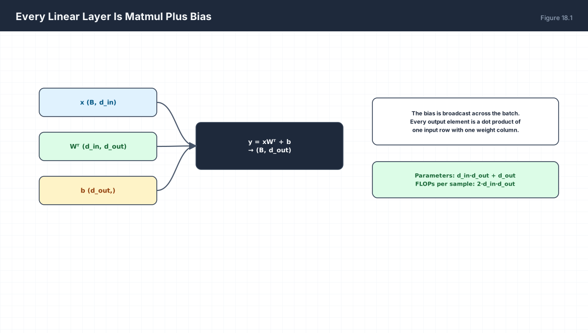
y = x Wᵀ + b

x   (B, d_in)
W   (d_out, d_in)     ← PyTorch's nn.Linear convention
Wᵀ  (d_in, d_out)
b   (d_out,)          broadcast across B
y   (B, d_out)

Parameters:  d_in·d_out + d_out
FLOPs/sample: 2·d_in·d_out      (multiply + add)
import numpy as np

B, d_in, d_out = 8, 768, 256
rng = np.random.default_rng(0)

x = rng.normal(size=(B, d_in))
W = rng.normal(size=(d_out, d_in)) * 0.02
b = np.zeros(d_out)

y = x @ W.T + b
print("y shape:", y.shape)                    # (8, 256)
assert y.shape == (B, d_out)

print("parameters:", W.size + b.size)         # 768*256 + 256
print("FLOPs/sample:", 2 * d_in * d_out)

# a single output element is a dot product of one input row with one weight row
assert np.isclose(y[0, 5], x[0] @ W[5] + b[5])
print("each output = one row · one weight row")
Nothing here is specific to a framework. nn.Linear stores the weight transposed relative to the mathematical convention, which is why the forward pass is written xWᵀ and not Wx — the latter is the per-sample form, the former handles a batch without a loop.
3. Normalisation Is Rescaling by Statistics
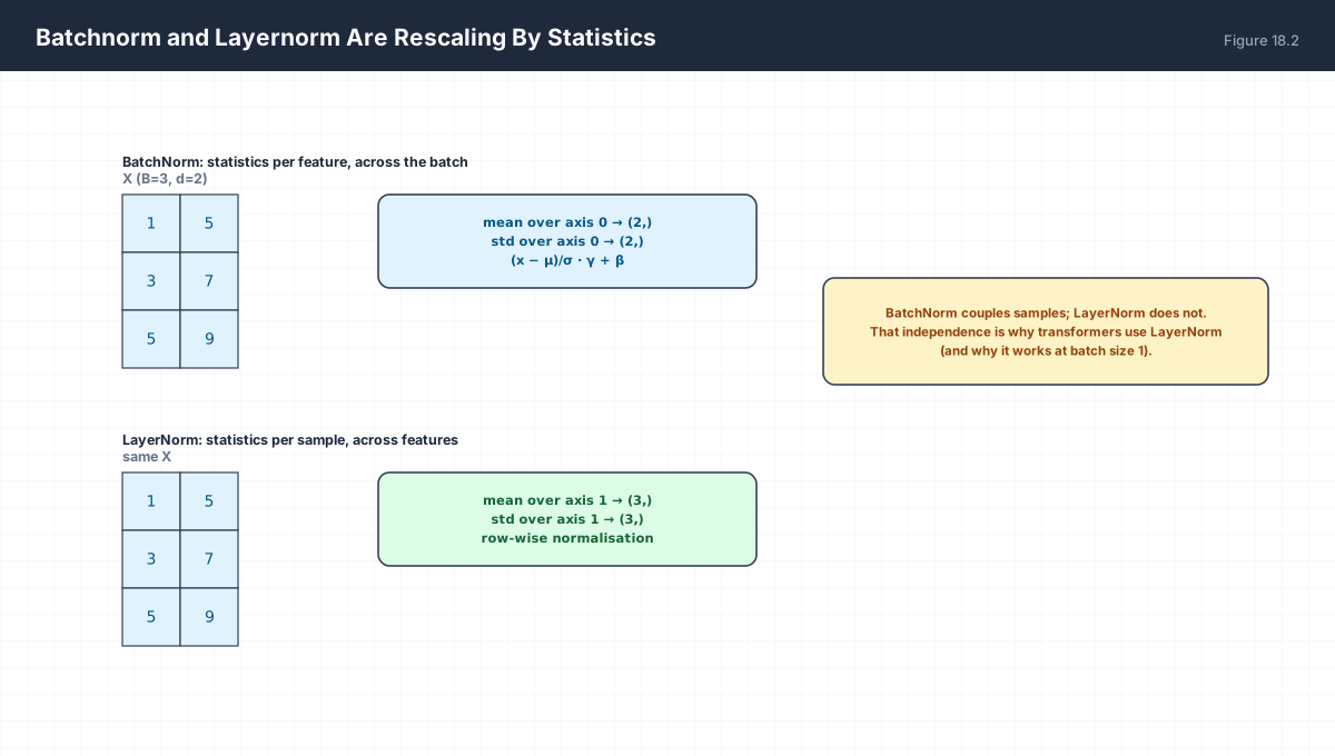
| Norm | Statistics Over | Shape of μ, σ | Couples Samples? |
|---|---|---|---|
| BatchNorm | the batch axis | (d,) per feature |
Yes |
| LayerNorm | the feature axis | (B,) per sample |
No |
| RMSNorm | feature axis, no mean subtraction | (B,) |
No |
import numpy as np

X = np.array([[1.0, 5.0], [3.0, 7.0], [5.0, 9.0]])   # (B=3, d=2)

def batchnorm(x, eps=1e-5):
    mu = x.mean(axis=0, keepdims=True)               # (1, d)
    var = x.var(axis=0, keepdims=True)
    return (x - mu) / np.sqrt(var + eps)

def layernorm(x, eps=1e-5):
    mu = x.mean(axis=1, keepdims=True)               # (B, 1)
    var = x.var(axis=1, keepdims=True)
    return (x - mu) / np.sqrt(var + eps)

bn = batchnorm(X)
ln = layernorm(X)
print("batchnorm column means:", np.round(bn.mean(axis=0), 10))   # ~0 per column
print("layernorm row means   :", np.round(ln.mean(axis=1), 10))   # ~0 per row
assert np.allclose(bn.mean(axis=0), 0.0, atol=1e-6)
assert np.allclose(ln.mean(axis=1), 0.0, atol=1e-6)
The coupling distinction is the practical one. BatchNorm computes statistics that depend on the other samples in the batch, so its behaviour changes between training and inference and it degrades at small batch sizes. LayerNorm uses only the current sample’s own features, so it behaves identically at batch size 1 and requires no running statistics — which is exactly why transformers use it.
4. Attention Is Three Projections and a Softmax
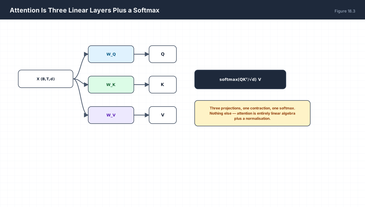
Q = X W_Q        (B, T, d) → (B, T, d)
K = X W_K
V = X W_V

S = Q Kᵀ / √d              (B, T, T)      scores, one per query-key pair
A = softmax(S, axis=-1)    (B, T, T)      each row sums to 1
O = A V                    (B, T, d)      weighted sum of value vectors

Per head, then concatenate heads and project with W_O.
import numpy as np

def softmax(z):
    z = z - z.max(axis=-1, keepdims=True)
    e = np.exp(z)
    return e / e.sum(axis=-1, keepdims=True)

B, T, d = 2, 6, 32
rng = np.random.default_rng(0)
X = rng.normal(size=(B, T, d))
Wq = rng.normal(size=(d, d)) * 0.1
Wk = rng.normal(size=(d, d)) * 0.1
Wv = rng.normal(size=(d, d)) * 0.1

Q, K, V = X @ Wq, X @ Wk, X @ Wv
S = (Q @ K.swapaxes(-1, -2)) / np.sqrt(d)
A = softmax(S)
O = A @ V

print("Q,K,V:", Q.shape, " S:", S.shape, " A:", A.shape, " O:", O.shape)
assert S.shape == (B, T, T) and O.shape == (B, T, d)
assert np.allclose(A.sum(axis=-1), 1.0)
print("attention row sums:", np.round(A.sum(axis=-1)[0], 6))
Every shape here is forced by Chapter 16’s rules. Kᵀ here means swapaxes(-1,-2) — transposing only the last two axes so the batch axes pass through untouched. The softmax runs over the last axis because that is the key axis, which is why each query’s attention weights form a distribution over positions.
5. Backpropagation Is Two Matrix Products
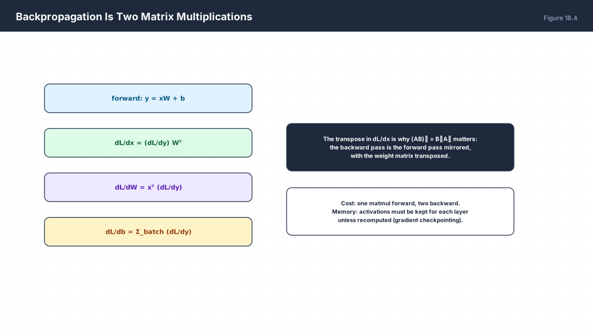
Forward:
  y  = x Wᵀ + b

Given dL/dy:
  dL/dx  = (dL/dy) W                 ← (B,d_out)(d_out,d_in) = (B,d_in)
  dL/dW  = (dL/dy)ᵀ x                ← (d_out,B)(B,d_in)    = (d_out,d_in)
  dL/db  = Σ_batch (dL/dy)           ← (d_out,)

The transposes are the (AB)ᵀ = BᵀAᵀ rule from Chapter 10.
import numpy as np

B, d_in, d_out = 4, 6, 3
rng = np.random.default_rng(1)
x = rng.normal(size=(B, d_in))
W = rng.normal(size=(d_out, d_in))
dL_dy = rng.normal(size=(B, d_out))

# analytic gradients
dL_dx = dL_dy @ W                       # (B, d_in)
dL_dW = dL_dy.T @ x                     # (d_out, d_in)
dL_db = dL_dy.sum(axis=0)               # (d_out,)

print("dx:", dL_dx.shape, " dW:", dL_dW.shape, " db:", dL_db.shape)
assert dL_dx.shape == (B, d_in) and dL_dW.shape == (d_out, d_in)

# numeric check on one weight
eps = 1e-6
W2 = W.copy()
W2[1, 2] += eps
loss_plus = np.sum(dL_dy * (x @ W2.T))
W3 = W.copy()
W3[1, 2] -= eps
loss_minus = np.sum(dL_dy * (x @ W3.T))
numeric = (loss_plus - loss_minus) / (2 * eps)
print("analytic vs numeric dW[1,2]:", round(dL_dW[1, 2], 6), round(numeric, 6))
assert np.isclose(dL_dW[1, 2], numeric, atol=1e-6)
The numeric check is the definitive test. If your analytic gradient disagrees with a central difference, the analytic gradient is wrong — which is exactly what torch.autograd.gradcheck automates.
6. Seven Operations, Repeated at Scale

| # | Operation | Expression | Chapter |
|---|---|---|---|
| 1 | Embedding lookup | E[token_ids] |
7 |
| 2 | Linear projection | xWᵀ + b |
10 |
| 3 | Score contraction | QKᵀ/√d |
8 |
| 4 | Softmax normalisation | softmax(S, -1) |
4 |
| 5 | Value blend | AV |
5 |
| 6 | Normalisation | (x−μ)/σ·γ+β |
11 |
| 7 | Residual add | x + f(x) |
8 |
7. Worked Examples
7.1 Parameters in one layer
nn.Linear(768, 256):
  weights  768·256 = 196,608
  bias           256
  total      196,864
7.2 Attention FLOPs
B=8, T=1024, d=768:
  QKV projections : 3 · 2·B·T·d·d ≈ 3.9e10
  scores          : 2·B·T²·d     ≈ 1.3e10
  value blend     : 2·B·T²·d     ≈ 1.3e10
Attention cost grows as T² — the reason context length is expensive.
7.3 Which axis does the norm use?
Input (B, T, d):
  BatchNorm  → reduce over (B, T), one μ per feature → shape (d,)
  LayerNorm  → reduce over d,        one μ per token  → shape (B, T, 1)
7.4 Gradient shape check
If W is (d_out, d_in) and x is (B, d_in):
  dL/dW must be (d_out, d_in) — same shape as W.
  A gradient whose shape differs from its parameter is always a bug.
7.5 Why the residual prevents collapse
y = x + f(x)
∂y/∂x = I + ∂f/∂x
The identity term means the gradient always has a path
straight through, regardless of how small ∂f/∂x becomes.
8. Verify It in Python
import numpy as np

rng = np.random.default_rng(0)

# --- 1. linear layer shapes and parameter count -------------------
B, d_in, d_out = 8, 768, 256
x = rng.normal(size=(B, d_in))
W = rng.normal(size=(d_out, d_in)) * 0.02
b = np.zeros(d_out)
y = x @ W.T + b
assert y.shape == (B, d_out)
assert W.size + b.size == d_in * d_out + d_out
print("params:", W.size + b.size, " out:", y.shape)

# --- 2. one output is a dot product -------------------------------
assert np.isclose(y[0, 3], x[0] @ W[3] + b[3])
print("output element == row dot weight row")

# --- 3. BatchNorm reduces over the batch axis ---------------------
X = np.array([[1., 5.], [3., 7.], [5., 9.]])
bn = (X - X.mean(axis=0, keepdims=True)) / np.sqrt(X.var(axis=0, keepdims=True) + 1e-5)
assert np.allclose(bn.mean(axis=0), 0.0, atol=1e-6)
print("batchnorm: zero column means")

# --- 4. LayerNorm reduces over the feature axis -------------------
ln = (X - X.mean(axis=1, keepdims=True)) / np.sqrt(X.var(axis=1, keepdims=True) + 1e-5)
assert np.allclose(ln.mean(axis=1), 0.0, atol=1e-6)
print("layernorm: zero row means")

# --- 5. attention end-to-end --------------------------------------
def softmax(z):
    z = z - z.max(axis=-1, keepdims=True)
    e = np.exp(z)
    return e / e.sum(axis=-1, keepdims=True)

Bs, T, dd = 2, 5, 16
Xs = rng.normal(size=(Bs, T, dd))
Wq, Wk, Wv = (rng.normal(size=(dd, dd)) * 0.2 for _ in range(3))
Q, K, V = Xs @ Wq, Xs @ Wk, Xs @ Wv
S = (Q @ K.swapaxes(-1, -2)) / np.sqrt(dd)
A = softmax(S)
O = A @ V
assert S.shape == (Bs, T, T) and O.shape == (Bs, T, dd)
assert np.allclose(A.sum(axis=-1), 1.0)
print("attention:", S.shape, "->", O.shape)

# --- 6. causal mask keeps rows normalised -------------------------
mask = np.triu(np.ones((T, T)), k=1).astype(bool)
S_masked = np.where(mask, -np.inf, S)
A_masked = softmax(S_masked)
assert np.allclose(A_masked.sum(axis=-1), 1.0)
assert np.allclose(np.triu(A_masked, k=1), 0.0)
print("causal mask: upper triangle zero, rows still sum to 1")

# --- 7. backprop gradients, checked numerically -------------------
Bb, di, do = 4, 6, 3
xb = rng.normal(size=(Bb, di))
Wb = rng.normal(size=(do, di))
dL_dy = rng.normal(size=(Bb, do))

dL_dx = dL_dy @ Wb
dL_dW = dL_dy.T @ xb
assert dL_dx.shape == xb.shape and dL_dW.shape == Wb.shape

eps = 1e-6
W_plus, W_minus = Wb.copy(), Wb.copy()
W_plus[0, 1] += eps
W_minus[0, 1] -= eps
num = (np.sum(dL_dy * (xb @ W_plus.T)) - np.sum(dL_dy * (xb @ W_minus.T))) / (2 * eps)
assert np.isclose(dL_dW[0, 1], num, atol=1e-6)
print("analytic dW matches numeric:", round(dL_dW[0, 1], 6))

# --- 8. residual gradient never vanishes --------------------------
dL_dx_via_residual = 1.0 + 0.0            # I + df/dx with df/dx = 0
assert dL_dx_via_residual == 1.0
print("residual keeps an identity gradient path")
print("all assertions passed")
9. Practice Questions
- Write a linear layer for
(B,512)→(B,128)with explicit shapes and parameter count. - Why does
nn.Linearstore the weight as(out, in)rather than(in, out)? - State which axis BatchNorm reduces over for a
(B,T,d)input, and the shape of μ. - Why is LayerNorm preferred in transformers over BatchNorm?
- Write the attention computation as five lines and give every shape.
- Why is
swapaxes(-1,-2)used instead of.T? - Derive
dL/dxanddL/dWfory = xWᵀ. - Why must a gradient have the same shape as its parameter?
- Explain in one line why
y = x + f(x)prevents vanishing gradients. - Give the asymptotic FLOPs of attention in
Tand explain the practical consequence.
10. Official References & Further Reading
Continue the Course
- Course Index: AI Mathematics Masterclass — All 48 Chapters
- Previous Chapter: Chapter 17: Determinants, Inverses & Numerical Conditioning
- Next Chapter: Chapter 19: Derivatives & Differentiation Rules
- Related Series: PyTorch Engineering Masterclass — All 16 Modules