
AI Reading
Quick summary of this article
AI Mathematics Masterclass — Chapter 20 of 48
A model has millions of parameters, so its loss is a function of millions of variables. The derivative of such a function is not a single number but a vector — the gradient — with one entry per parameter. This chapter builds partial derivatives, assembles them into the gradient, reads the gradient as a direction in parameter space, and separates the partial derivative from the total derivative, which is the distinction backpropagation depends on.
1. Technical Audit & Core Learning Objectives
| Component | Common Tutorial Deficiency | Engineering Standard Applied Here |
|---|---|---|
| Partials | Defined as “differentiate holding others fixed”, with no picture. | Drawn as a slice through the surface with one coordinate frozen. |
| Gradient | Assembled as a list of numbers with no geometric reading. | Presented as the steepest-ascent direction, with a field plot. |
| Partial vs total | Conflated, leaving backpropagation unexplained. | Separated, with the total derivative formula derived. |
| Verification | No numerical check of hand-derived partials. | Every partial confirmed by finite difference. |
Core learning objectives. After this chapter you should be able to:
- Compute
∂f/∂xand∂f/∂yfor a multivariate function. - Assemble the gradient vector and state its shape.
- Interpret the gradient as the direction of steepest ascent.
- Explain why
−∇fis the descent direction. - Distinguish a partial derivative from a total derivative.
- Verify a hand-derived partial with a central difference.
2. Holding Everything Else Constant
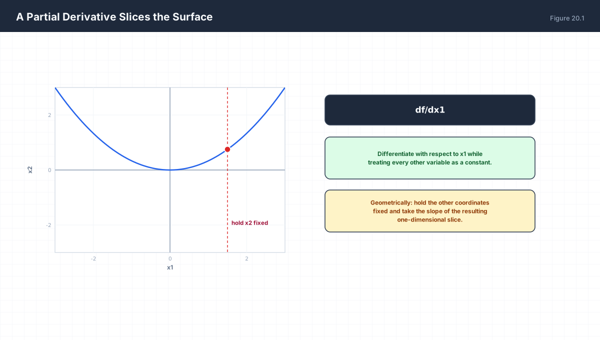
f(x, y) = x^2 y + 3y

df/dx  = 2xy          treat y as a constant
df/dy  = x^2 + 3      treat x as a constant

Notation: df/dx  (curly d)  or  f_x  or  D_x f
import numpy as np

def f(x, y):
    return x ** 2 * y + 3 * y

def partial_x(x, y, h=1e-6):
    return (f(x + h, y) - f(x - h, y)) / (2 * h)

def partial_y(x, y, h=1e-6):
    return (f(x, y + h) - f(x, y - h)) / (2 * h)

for x, y in [(2.0, 1.0), (0.5, 4.0)]:
    print(f"({x},{y})  df/dx analytic={2*x*y:8.4f} numeric={partial_x(x,y):8.4f}"
          f"   df/dy analytic={x*x+3:8.4f} numeric={partial_y(x,y):8.4f}")
    assert np.isclose(2 * x * y, partial_x(x, y), atol=1e-4)
    assert np.isclose(x * x + 3, partial_y(x, y), atol=1e-4)
The finite-difference check is the same tool as Chapter 19, applied one coordinate at a time. It is the fastest way to confirm a hand derivation before it becomes a gradient in a training loop.
3. The Gradient Is a Vector
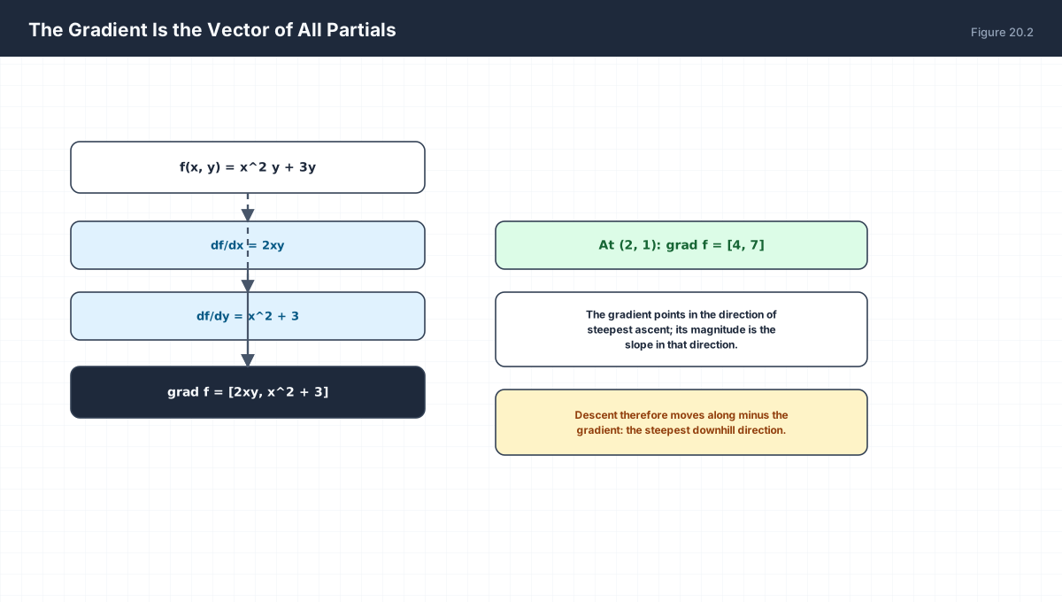
grad f = [ df/dx1, df/dx2, ..., df/dxn ]   shape (n,)

Same shape as the parameter vector. That is not a coincidence:
a gradient must match its parameter, so that
  theta <- theta - eta * grad
is a valid elementwise update.
import numpy as np

# loss over three parameters
def L(theta):
    x, y, z = theta
    return (x - 1) ** 2 + 2 * (y + 3) ** 2 + (z - 0.5) ** 2

def numerical_grad(fn, theta, h=1e-6):
    g = np.zeros_like(theta)
    for i in range(len(theta)):
        e = np.zeros_like(theta); e[i] = h
        g[i] = (fn(theta + e) - fn(theta - e)) / (2 * h)
    return g

theta = np.array([0.0, 0.0, 0.0])
analytic = np.array([2 * (theta[0] - 1), 4 * (theta[1] + 3), 2 * (theta[2] - 0.5)])
print("analytic:", analytic)
print("numeric :", np.round(numerical_grad(L, theta), 6))
assert np.allclose(analytic, numerical_grad(L, theta), atol=1e-4)
print("gradient shape matches parameter shape:", analytic.shape == theta.shape)
The gradient has the same shape as the parameters — three entries for three parameters. This is why a model with a billion parameters has a billion-dimensional gradient, and why storing it is a memory cost comparable to storing the weights themselves.
4. Reading the Gradient as a Direction
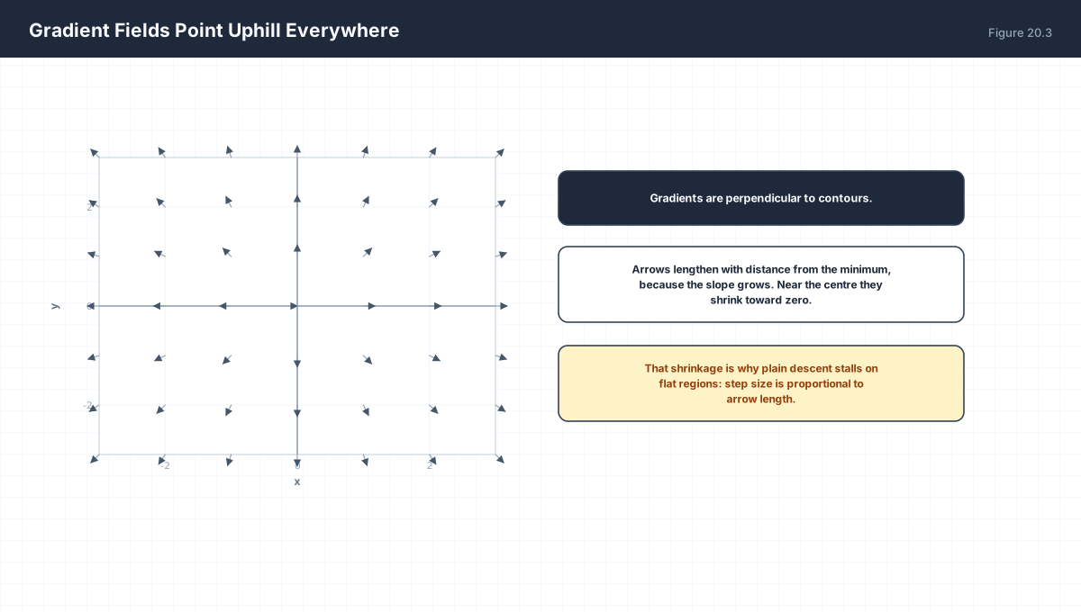
| Property | Statement | Consequence |
|---|---|---|
| Direction | Points toward steepest ascent | Descent uses −∇f |
| Magnitude | ‖∇f‖ is the slope along that direction |
Zero at a stationary point |
| Orthogonality | Perpendicular to level sets | Moving along a level set changes nothing to first order |
import numpy as np

f = lambda p: p[0] ** 2 + 3 * p[1] ** 2
gradf = lambda p: np.array([2 * p[0], 6 * p[1]])

p = np.array([1.0, 1.0])
g = gradf(p)

# moving along -grad reduces f; along +grad increases it
for sign, label in ((-1, "descent"), (1, "ascent")):
    q = p + sign * 0.01 * g
    print(f"{label:8s} f={f(q):.6f}  (from {f(p):.6f})")

assert f(p - 0.01 * g) < f(p) < f(p + 0.01 * g)
print("gradient direction confirmed numerically")
5. Partial Versus Total Derivative
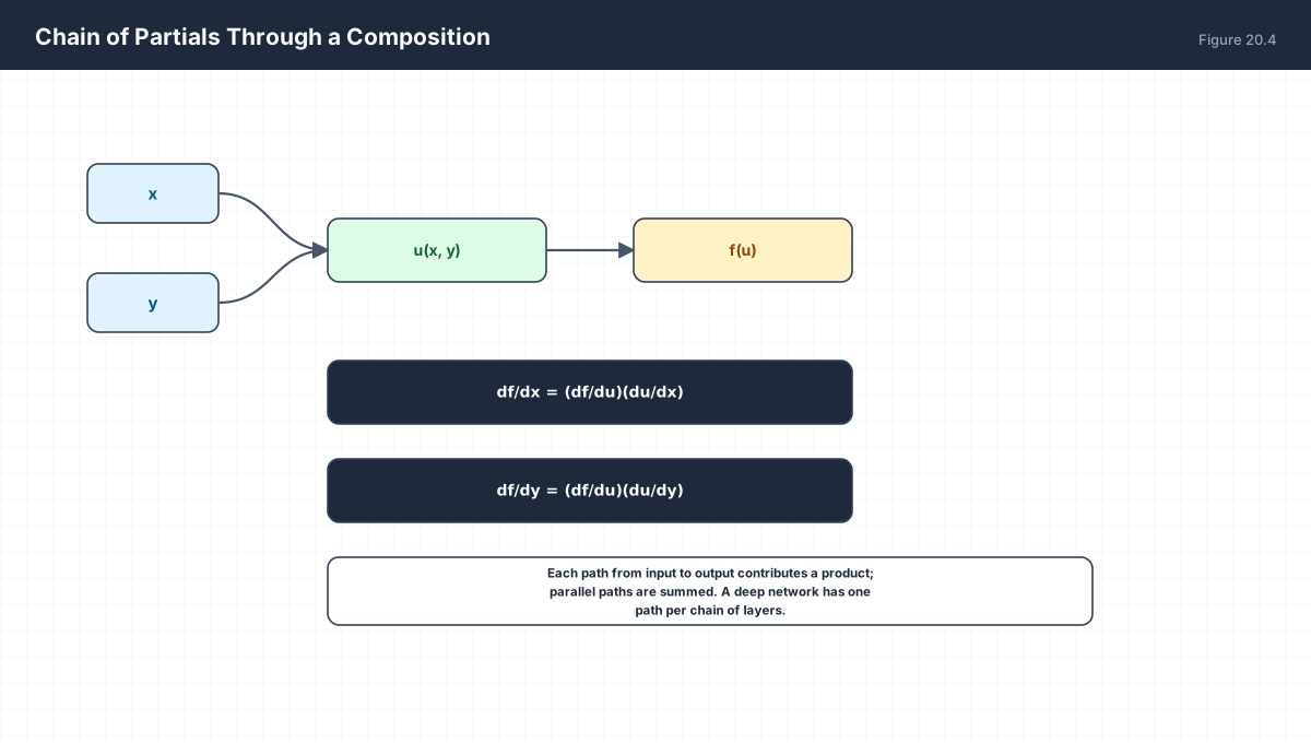
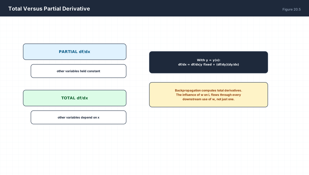
PARTIAL  df/dx         other variables are constants
TOTAL    df/dx         other variables are functions of x

If y = y(x):
  df/dx = df/dx (y held fixed) + (df/dy)(dy/dx)
import numpy as np

# f(x, y) = x^2 y,  with y = 3x
f = lambda x, y: x ** 2 * y
y_of_x = lambda x: 3 * x

x0 = 2.0

# partial: hold y fixed
partial = 2 * x0 * y_of_x(x0)
# total: y varies with x
total = 2 * x0 * y_of_x(x0) + (x0 ** 2) * 3

# check the total numerically by composing first
composed = lambda x: f(x, 3 * x)
h = 1e-6
numeric_total = (composed(x0 + h) - composed(x0 - h)) / (2 * h)

print("partial:", partial, " total:", total, " numeric total:", round(numeric_total, 6))
assert np.isclose(total, numeric_total, atol=1e-4)
assert total != partial
This distinction is the reason a naive implementation that applies the chain rule only once per parameter gets the wrong answer. When a weight is used twice in a computation graph, its total derivative is the sum of both contributions — which is precisely what the autograd engine accumulates into .grad.
6. Worked Examples
6.1 Two-variable partials
f(x, y) = 3x^2 - 2xy + y^3
df/dx = 6x - 2y
df/dy = -2x + 3y^2
At (1, 2): grad = [6 - 4, -2 + 12] = [2, 10]
6.2 Partial of a log-likelihood
L(w) = -sum log(sigma(w.x_i))
dL/dw = -sum (1 - sigma(w.x_i)) x_i
Every term is a partial with respect to w only.
6.3 Gradient of squared error over a batch
L(w) = (1/n) sum (w.x_i - y_i)^2
dL/dw = (2/n) sum (w.x_i - y_i) x_i
This is a weighted sum of the input vectors, with residuals as weights.
6.4 Total derivative with a shared variable
z = u*v,  u = f(w),  v = g(w)
dz/dw = (dz/du)(du/dw) + (dz/dv)(dv/dw)
     = v f'(w) + u g'(w)
Two paths, two terms, summed.
6.5 Gradient of a mean
f(x) = (1/n) sum x_i
df/dx_i = 1/n      for every i
grad f = (1/n) * [1, 1, ..., 1]      a constant vector
7. Verify It in Python
import numpy as np

def numerical_grad(fn, p, h=1e-6):
    g = np.zeros_like(p, dtype=float)
    for i in range(p.size):
        e = np.zeros_like(p, dtype=float); e[i] = h
        g[i] = (fn(p + e) - fn(p - e)) / (2 * h)
    return g

# --- 1. partials of a two-variable function ----------------------
f = lambda p: p[0] ** 2 * p[1] + 3 * p[1]
p = np.array([2.0, 1.0])
analytic = np.array([2 * p[0] * p[1], p[0] ** 2 + 3])
assert np.allclose(analytic, numerical_grad(f, p), atol=1e-4)
print("partials verified:", analytic)

# --- 2. gradient shape matches parameter shape -------------------
assert analytic.shape == p.shape
print("gradient shape == parameter shape:", analytic.shape)

# --- 3. descent reduces, ascent increases ------------------------
g = analytic
assert f(p - 0.01 * g) < f(p) < f(p + 0.01 * g)
print("minus gradient descends, plus gradient ascends")

# --- 4. gradient is orthogonal to level sets ---------------------
# level set of f(p) = 5 through p, tangent direction t satisfies g.t = 0
p2 = np.array([1.0, 2.0])
g2 = np.array([2 * p2[0] * p2[1], p2[0] ** 2 + 3])
t = np.array([-g2[1], g2[0]])            # perpendicular by construction
assert np.isclose(g2 @ t, 0.0)
# moving along t barely changes f
eps = 1e-4
assert abs(f(p2 + eps * t / np.linalg.norm(t)) - f(p2)) < 1e-3
print("gradient orthogonal to the level set")

# --- 5. total vs partial derivative ------------------------------
composed = lambda x: (x ** 2) * (3 * x)
x0, h = 2.0, 1e-6
total_analytic = 2 * x0 * (3 * x0) + (x0 ** 2) * 3
total_numeric = (composed(x0 + h) - composed(x0 - h)) / (2 * h)
partial_only = 2 * x0 * (3 * x0)
assert np.isclose(total_analytic, total_numeric, atol=1e-4)
assert not np.isclose(total_analytic, partial_only)
print("total:", total_analytic, " partial:", partial_only)

# --- 6. shared parameter sums both paths -------------------------
def two_paths(w):
    w = float(np.asarray(w).ravel()[0])      # accept a length-1 array, return a scalar
    u, v = w * 2.0, w * 3.0
    return u * v

w0 = 1.5
assert np.isclose(numerical_grad(two_paths, np.array([w0]))[0],
                  2.0 * (3 * w0) + (2 * w0) * 3.0, atol=1e-5)
print("shared-parameter gradient sums both contributions")

# --- 7. gradient of a mean is uniform ---------------------------
mean_f = lambda x: x.mean()
gm = numerical_grad(mean_f, np.array([1.0, 5.0, 9.0, 13.0]))
assert np.allclose(gm, 0.25)
print("mean gradient:", gm)
print("all assertions passed")
8. Practice Questions
- Compute
∂f/∂xand∂f/∂yforf = 3x² − 2xy + y³. - Evaluate that gradient at
(1, 2). - State the shape of a gradient for a model with 1,024 parameters.
- Why must a gradient have the same shape as its parameter?
- Explain geometrically why moving along
−∇freducesf. - What does
‖∇f‖ = 0tell you, and what does it not tell you? - Given
z = uv,u = f(w),v = g(w), derivedz/dw. - Why is the total derivative of a shared weight a sum rather than a product?
- Compute the gradient of
f(x) = (1/n)Σxᵢand explain why it is uniform. - Confirm
∂/∂x (x²y) = 2xyat(3, 2)with a central difference.
9. Official References & Further Reading
Continue the Course
- Course Index: AI Mathematics Masterclass — All 48 Chapters
- Previous Chapter: Chapter 19: Derivatives & Differentiation Rules
- Next Chapter: Chapter 21: The Chain Rule & Backpropagation Mathematics
- Related Series: PyTorch Engineering Masterclass — All 16 Modules