
AI Reading
Quick summary of this article
AI Mathematics Masterclass — Chapter 22 of 48
A gradient tells you which direction is downhill. It does not tell you how far to step, whether the surface curves up or down, or whether you are standing in a narrow ravine. That information lives in the second derivative — aggregated into the Hessian for many variables, and into the Jacobian for vector-valued functions. This chapter builds both, explains why the Hessian’s eigenvalues set a hard ceiling on the learning rate, and shows the approximations that make second-order reasoning affordable at model scale.
1. Technical Audit & Core Learning Objectives
| Component | Common Tutorial Deficiency | Engineering Standard Applied Here |
|---|---|---|
| Jacobian | Defined as a matrix of symbols with no use. | Positioned as the general case of which a gradient is one row. |
| Hessian | Written out and then abandoned as impractical. | Its eigenvalues used to explain the learning-rate ceiling and valley slowdown. |
| Curvature types | Minimum/maximum/saddle named without a test. | Classified from the eigenvalue signs, with a saddle drawn correctly. |
| Approximations | Never mentioned, leaving second-order methods as theory. | Diagonal, Gauss–Newton, and Adam’s second moment all explained as approximations. |
Core learning objectives. After this chapter you should be able to:
- Write the Jacobian of
f: ℝⁿ → ℝᵐand state its shape. - Recognise a gradient as a special case of a Jacobian.
- Construct and read a Hessian, and use symmetry.
- Classify a stationary point from Hessian eigenvalue signs.
- Derive the stability condition
η < 2/λmax. - Explain diagonal and Gauss–Newton approximations and when each applies.
2. The Jacobian
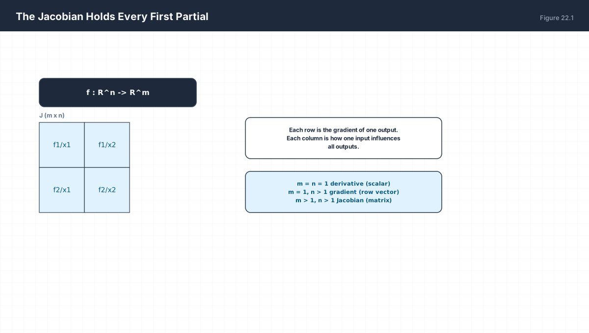
f : R^n -> R^m         J is (m x n)

J[i, j] = df_i / dx_j

m = 1        J is a single row  ->  the gradient, transposed
m = n = 1    J is a single entry -> the ordinary derivative
import numpy as np

def jacobian(fn, x, h=1e-6):
    """Numerical Jacobian of fn: R^n -> R^m."""
    x = np.asarray(x, dtype=float)
    f0 = np.atleast_1d(fn(x))
    J = np.zeros((f0.size, x.size))
    for j in range(x.size):
        e = np.zeros_like(x); e[j] = h
        J[:, j] = (np.atleast_1d(fn(x + e)) - np.atleast_1d(fn(x - e))) / (2 * h)
    return J

# f(x) = [x1^2, x1*x2, x2^3]
f = lambda v: np.array([v[0] ** 2, v[0] * v[1], v[1] ** 3])
x = np.array([2.0, 3.0])
J = jacobian(f, x)
print("J =\n", np.round(J, 6))

analytic = np.array([[2 * x[0], 0.0],
                     [x[1], x[0]],
                     [0.0, 3 * x[1] ** 2]])
assert np.allclose(J, analytic, atol=1e-4)
print("shape:", J.shape, " (m x n) =", (3, 2))
The Jacobian is what you get when a function has vector output. A gradient is the special case with scalar output, which is why a gradient is shape (n,) while a Jacobian for m outputs is (m, n) — and why computing full Jacobians in a network with a million outputs would be prohibitive.
3. The Hessian
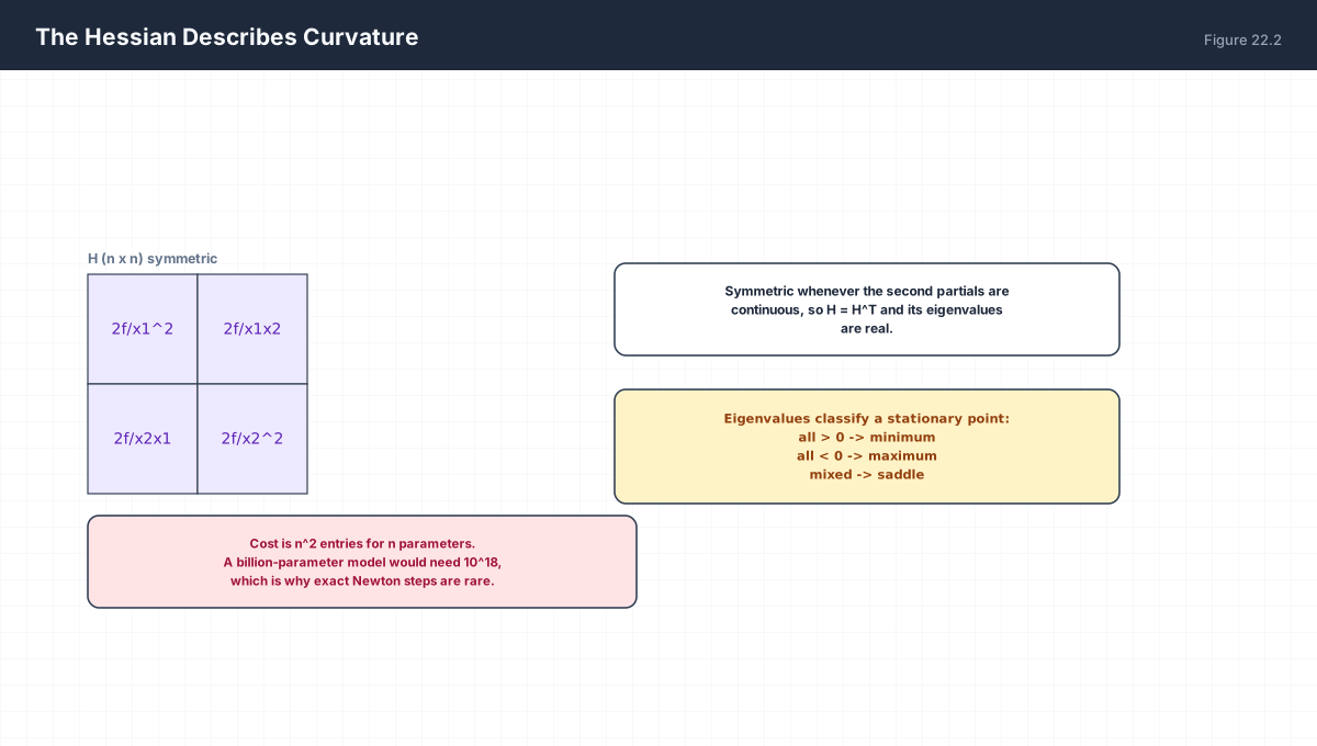
H[i, j] = d2f / dx_i dx_j          H is (n x n)

Symmetric when second partials are continuous (H = H^T)
Eigenvalues are then real.

Classification at a stationary point:
  all lambda > 0   minimum
  all lambda < 0   maximum
  mixed signs      saddle
  any lambda = 0   degenerate, test inconclusive
import numpy as np

# f(x, y) = x^2 + 4y^2  -> Hessian is constant
H = np.array([[2.0, 0.0], [0.0, 8.0]])
evals = np.linalg.eigvalsh(H)
print("eigenvalues:", evals, "-> minimum:", np.all(evals > 0))

# f(x, y) = x^2 - y^2  -> saddle
H2 = np.array([[2.0, 0.0], [0.0, -2.0]])
ev2 = np.linalg.eigvalsh(H2)
print("eigenvalues:", ev2, "-> indefinite:", np.any(ev2 > 0) and np.any(ev2 < 0))

# a coupled case: second partials interact
# f = x^2 + xy + y^2
H3 = np.array([[2.0, 1.0], [1.0, 2.0]])
ev3 = np.linalg.eigvalsh(H3)
print("coupled eigenvalues:", np.round(ev3, 4), "-> minimum:", np.all(ev3 > 0))
print("symmetric:", np.allclose(H3, H3.T))
4. Curvature Determines the Shape
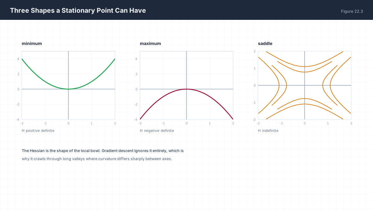
| Eigenvalues | Shape | Gradient Descent Behaviour |
|---|---|---|
| all positive | bowl | attracted from every direction |
| all negative | dome | repelled along every direction |
| mixed | saddle | attracted along some axes, repelled along others |
Saddles matter more than local minima in high dimensions. For a random critical point in n dimensions, the chance that all n eigenvalues share a sign is roughly 2^(1−n) — vanishingly small. Almost every stationary point a deep network encounters is a saddle, which is why the "stuck in a local minimum" explanation for stalled training is usually wrong: the gradient is small because of flat directions, not because of a trap.
5. Why Curvature Caps the Learning Rate
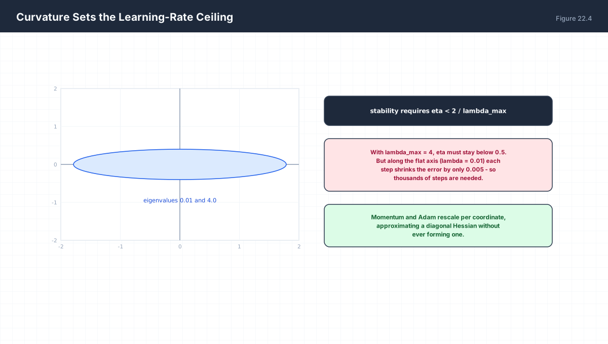
For a quadratic with curvature lambda, descent is stable only if
  eta < 2 / lambda_max

One step along an eigen-direction with eigenvalue lambda gives
  error_new = (1 - eta lambda) * error_old

So:
  eta lambda < 1        error shrinks monotonically (fastest at 1)
  1 < eta lambda < 2    error alternates sign but still shrinks
  eta lambda > 2        error grows  -> divergence
import numpy as np

def run(lam, eta, steps=25):
    w = 1.0
    for _ in range(steps):
        w = w - eta * lam * w
    return w

for lam in (1.0, 4.0):
    for eta in (0.1, 0.4, 0.55):
        stable = eta * lam < 2
        print(f"lambda={lam:3.1f} eta={eta:4.2f}  eta*lambda={eta*lam:5.2f}"
              f"  w={run(lam, eta):+.3e}  {'' if stable else 'DIVERGED'}")
The consequence is the classic valley problem. If curvature is 0.01 along one axis and 4.0 along another, the learning rate must stay below 0.5 for stability — but at 0.5 the flat axis improves by only 0.5% per step. That factor of 400 between the two curvatures is the condition number of the Hessian, and it is the reason momentum and adaptive methods exist.
6. Approximations That Make This Practical
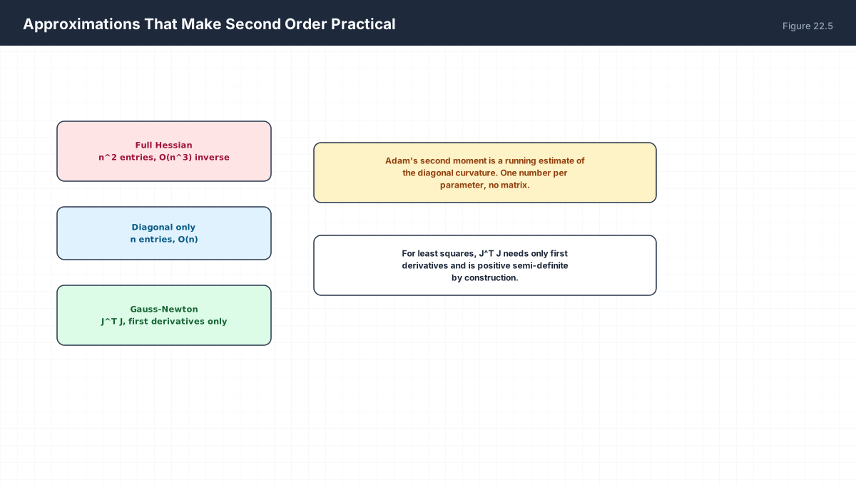
| Method | Storage | What It Captures |
|---|---|---|
| Full Hessian | n² |
All curvature, including cross-terms |
| Diagonal | n |
Per-axis curvature only |
Gauss–Newton JᵀJ |
n² |
Curvature from first derivatives; PSD by construction |
Adam's v |
n |
Running estimate of diagonal curvature from g² |
import numpy as np

# Gauss-Newton for least squares: H ~ J^T J
rng = np.random.default_rng(0)
X = rng.normal(size=(20, 3))
y = X @ np.array([1.0, -2.0, 0.5]) + rng.normal(0, 0.1, 20)

residual = lambda w: X @ w - y
J = X                                       # d(residual)/dw = X
H_gn = J.T @ J
print("Gauss-Newton H shape:", H_gn.shape)
print("symmetric:", np.allclose(H_gn, H_gn.T))
print("positive semi-definite:", np.all(np.linalg.eigvalsh(H_gn) >= -1e-9))

# the Gauss-Newton step solves it in one move for a linear model
w0 = np.zeros(3)
step = np.linalg.solve(H_gn, -J.T @ residual(w0))
print("one Newton step from zero:", np.round(w0 + step, 6))
7. Worked Examples
7.1 A constant Hessian
f(x,y) = x^2 + 9y^2
H = [[2, 0], [0, 18]]
eigenvalues 2 and 18 -> minimum
condition number 9 -> the valley is 9 times longer than wide
7.2 A saddle from a cubic
f(x,y) = x^2 - y^2
H = [[2, 0], [0, -2]]
eigenvalues +2, -2 -> mixed -> saddle at the origin
7.3 Coupled cross-terms
f(x,y) = x^2 + xy + y^2
H = [[2, 1], [1, 2]]
eigenvalues 1 and 3, both positive -> minimum
The off-diagonal 1 rotates the valley 45 degrees.
7.4 Stability limit
lambda_max = 8  ->  eta < 0.25
At eta = 0.24 each step multiplies error by |1 - 1.92| = 0.92
At eta = 0.26 each step multiplies error by |1 - 2.08| = 1.08  -> diverges
7.5 Jacobian of a linear layer
y = Wx,  W is (m, n)
dy/dx = W          the Jacobian is just the weight matrix
That is why linear layers have constant, cheap derivatives.
8. Verify It in Python
import numpy as np

# --- 1. numerical Jacobian matches analytic ----------------------
def jac(fn, x, h=1e-6):
    x = np.asarray(x, float)
    f0 = np.atleast_1d(fn(x))
    J = np.zeros((f0.size, x.size))
    for j in range(x.size):
        e = np.zeros_like(x); e[j] = h
        J[:, j] = (np.atleast_1d(fn(x + e)) - np.atleast_1d(fn(x - e))) / (2 * h)
    return J

f = lambda v: np.array([v[0] ** 2, v[0] * v[1], v[1] ** 3])
J = jac(f, np.array([2.0, 3.0]))
assert J.shape == (3, 2)
assert np.allclose(J, [[4, 0], [3, 2], [0, 27]], atol=1e-4)
print("Jacobian correct, shape", J.shape)

# --- 2. gradient is a one-row Jacobian ---------------------------
g_f = lambda v: np.array([v[0] ** 2 + v[1] ** 2])
Jg = jac(g_f, np.array([1.0, 2.0]))
assert Jg.shape == (1, 2)
print("scalar output -> 1-row Jacobian:", Jg)

# --- 3. Hessian symmetry and classification ----------------------
def hess(fn, x, h=1e-5):
    x = np.asarray(x, float)
    n = x.size
    Hm = np.zeros((n, n))
    for i in range(n):
        for j in range(n):
            e1 = np.zeros(n); e1[i] = h
            e2 = np.zeros(n); e2[j] = h
            Hm[i, j] = (fn(x + e1 + e2) - fn(x + e1 - e2)
                        - fn(x - e1 + e2) + fn(x - e1 - e2)) / (4 * h * h)
    return Hm

f2 = lambda v: v[0] ** 2 + 4 * v[1] ** 2
H = hess(f2, np.array([0.0, 0.0]))
assert np.allclose(H, [[2, 0], [0, 8]], atol=1e-2)
assert np.allclose(H, H.T)
assert np.all(np.linalg.eigvalsh(H) > 0)
print("Hessian verified, positive definite")

# --- 4. saddle detection -----------------------------------------
f3 = lambda v: v[0] ** 2 - v[1] ** 2
H3 = hess(f3, np.array([0.0, 0.0]))
ev = np.linalg.eigvalsh(H3)
assert np.any(ev > 0) and np.any(ev < 0)
print("saddle eigenvalues:", np.round(ev, 3))

# --- 5. learning-rate ceiling ------------------------------------
lam = 4.0
def run(eta, steps=60):
    w = 1.0
    for _ in range(steps):
        w = w - eta * lam * w
    return w

assert abs(run(0.2)) < 1e-6              # stable:  |1-0.8| = 0.2 per step
assert abs(run(0.6)) > 1e6               # unstable: |1-2.4| = 1.4 per step, 1.4^60 ≈ 6e8
print("stable at eta=0.2, diverges at eta=0.6")

# --- 6. Gauss-Newton equals the exact solution for a linear model -
rng = np.random.default_rng(1)
X = rng.normal(size=(30, 4))
y = X @ np.array([1.0, -2.0, 0.5, 3.0]) + rng.normal(0, 1e-10, 30)
w_gn = np.linalg.solve(X.T @ X, X.T @ y)
assert np.allclose(w_gn, [1.0, -2.0, 0.5, 3.0], atol=1e-6)
print("Gauss-Newton recovers exact weights:", np.round(w_gn, 6))

# --- 7. Hessian condition number == valley aspect ratio ---------
Hc = np.array([[2.0, 0.0], [0.0, 18.0]])
assert np.isclose(np.linalg.cond(Hc), 9.0)
print("Hessian condition number:", np.linalg.cond(Hc))
print("all assertions passed")
9. Practice Questions
- Write the Jacobian of
f(x,y) = [x²y, x + y]and give its shape. - Explain why a gradient is a Jacobian with one row.
- Compute the Hessian of
x² + xy + y²and its eigenvalues. - Classify the stationary point of
x² − y²and sketch the contours. - Why are Hessians symmetric, and what does that guarantee?
- Given
λmax = 10, what is the largest stable learning rate? - Explain the valley problem in terms of Hessian eigenvalues.
- Why is a random critical point in high dimensions almost always a saddle?
- What does Gauss–Newton approximate, and when is it exact?
- How many entries does a Hessian have for a model with 10⁶ parameters?
10. Official References & Further Reading
Continue the Course
- Course Index: AI Mathematics Masterclass — All 48 Chapters
- Previous Chapter: Chapter 21: The Chain Rule & Backpropagation Mathematics
- Next Chapter: Chapter 23: Gradient Descent, Momentum & Adaptive Optimizers
- Related Series: PyTorch Engineering Masterclass — All 16 Modules