
AI Reading
Quick summary of this article
AI Mathematics Masterclass — Chapter 25 of 48
Probability is the language machine learning uses to express uncertainty, and it rests on three axioms from which everything else follows. This chapter builds those axioms, turns them into the algebra of events, defines conditional probability as a restriction of the sample space, and shows why the difference between P(A|B) and P(B|A) is the single most consequential error in applied statistics.
1. Technical Audit & Core Learning Objectives
Probability chapters typically present a list of rules and then jump to distributions, leaving the reader unable to say why P(A|B) and P(B|A) differ or what independence actually asserts.
| Component | Common Tutorial Deficiency | Engineering Standard Applied Here |
|---|---|---|
| Axioms | Stated then abandoned; derived rules presented as equally fundamental. | Three axioms shown to generate the rest, so nothing is assumed twice. |
| Conditioning | Formula given without the “restricted universe” reading. | Drawn as renormalisation inside B, which makes the asymmetry obvious. |
| Independence | Conflated with uncorrelatedness and with causation. | Separated explicitly, with the language-model counterexample. |
| Marginalisation | Mentioned as a footnote. | Presented as the operation that makes exact inference expensive. |
Core learning objectives. After this chapter you should be able to:
- State the three Kolmogorov axioms and derive the complement rule from them.
- Apply inclusion–exclusion to compute
P(A ∪ B). - Compute conditional probabilities and explain the renormalisation.
- Test two events for independence and distinguish it from causation.
- Marginalise a joint distribution over an unwanted variable.
- Apply the chain rule to decompose a joint distribution.
2. Three Axioms
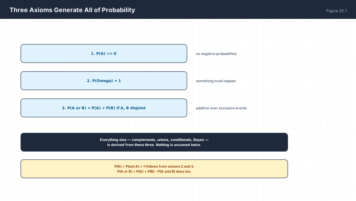
1.  P(A) >= 0                       non-negativity
2.  P(Omega) = 1                    normalisation
3.  P(A or B) = P(A) + P(B)         for disjoint A, B

From 2 and 3:  P(A) + P(not A) = 1
From 3:        P(A or B) = P(A) + P(B) - P(A and B)
import numpy as np

rng = np.random.default_rng(0)
n = 200_000
rolls = rng.integers(1, 7, n)

A = rolls <= 2          # {1, 2}
B = rolls % 2 == 0      # {2, 4, 6}

pA, pB = A.mean(), B.mean()
pAB = (A & B).mean()

print(f"P(A)={pA:.4f}  P(B)={pB:.4f}  P(A and B)={pAB:.4f}")
print(f"P(A or B) empirical={(A | B).mean():.4f}")
print(f"P(A) + P(B) - P(A and B) ={pA + pB - pAB:.4f}")
assert abs((A | B).mean() - (pA + pB - pAB)) < 0.005
print("inclusion-exclusion confirmed")
3. Events as Subsets
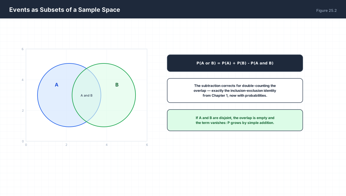
The inclusion–exclusion identity from Chapter 1 reappears here with probabilities instead of cardinalities. It is not a separate rule — it is what axiom 3 produces once you account for overlap.
| Operation | Set | Probability |
|---|---|---|
| complement | Aᶜ |
1 − P(A) |
| union | A ∪ B |
P(A) + P(B) − P(A ∩ B) |
| intersection | A ∩ B |
P(A) + P(B) − P(A ∪ B) |
4. Conditional Probability
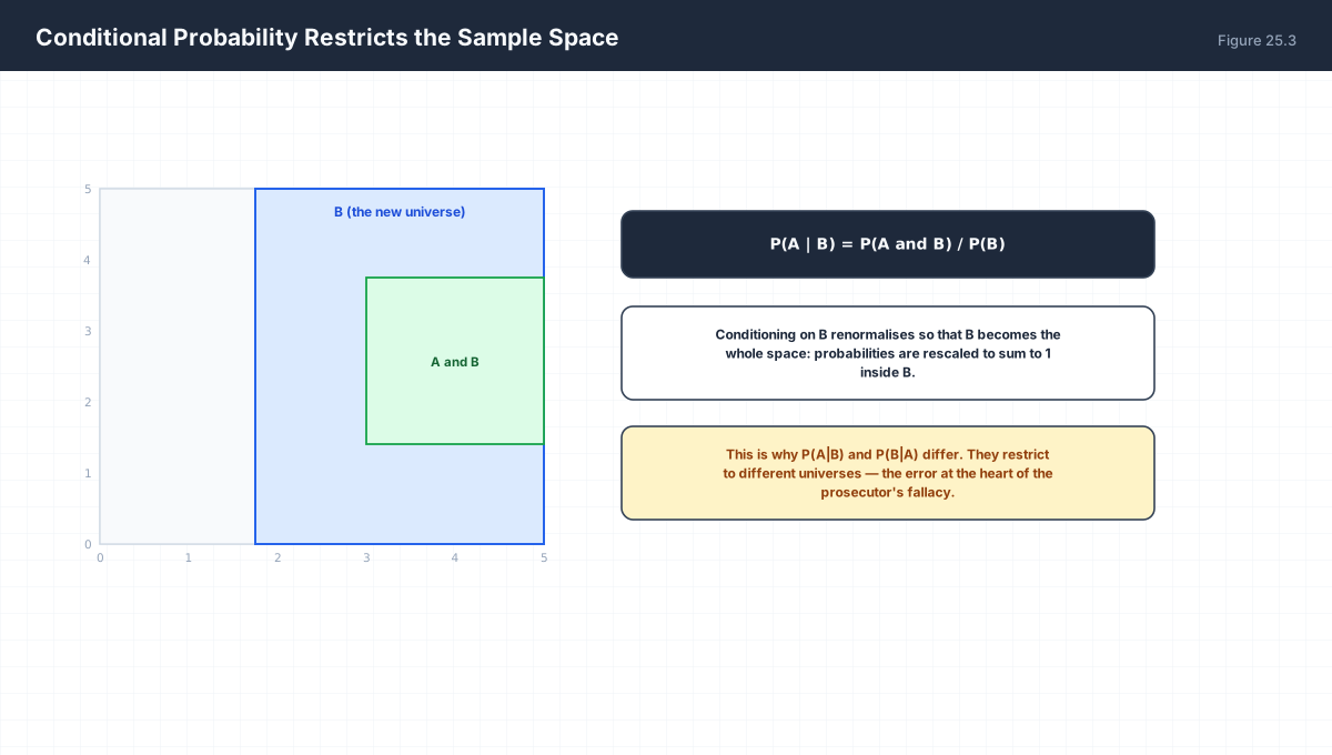
P(A | B) = P(A and B) / P(B)        provided P(B) > 0

Interpretation: the fraction of B's probability that also lies in A.

P(A|B) and P(B|A) are generally different, because they
restrict to different universes.
import numpy as np

rng = np.random.default_rng(1)
n = 500_000
# two binary features, correlated
u = rng.random(n)
x = (u < 0.3).astype(int)                    # feature X
y = np.where(u < 0.25, 1, (rng.random(n) < 0.2).astype(int))

p_x1 = x.mean()
p_y1 = y.mean()
p_both = ((x == 1) & (y == 1)).mean()

p_x_given_y = p_both / p_y1
p_y_given_x = p_both / p_x1

print(f"P(X=1)={p_x1:.4f}  P(Y=1)={p_y1:.4f}  P(both)={p_both:.4f}")
print(f"P(X=1|Y=1)={p_x_given_y:.4f}   P(Y=1|X=1)={p_y_given_x:.4f}")
assert abs(p_x_given_y - p_y_given_x) > 0.01
print("the two conditionals differ, as they should")
5. Independence
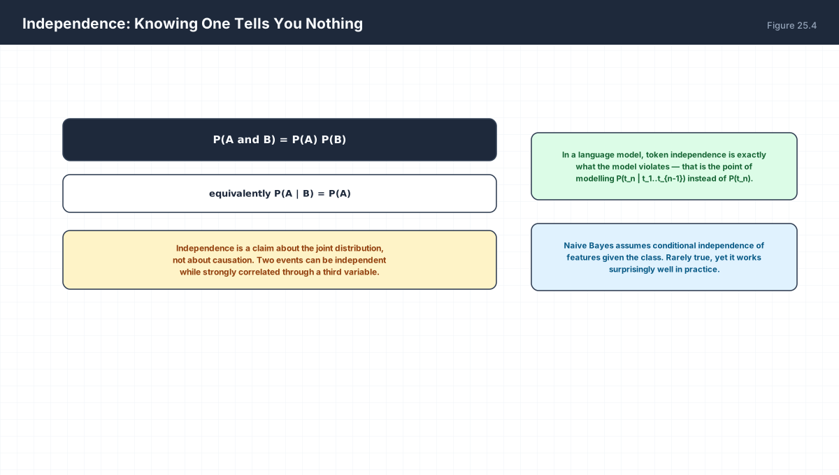
A and B independent  <=>  P(A and B) = P(A) P(B)
                     <=>  P(A | B) = P(A)

Caution: independence is not uncorrelatedness, and neither
implies causation. Two events can be independent given a
third variable and dependent without it (Simpson's paradox).
Independence is the assumption a language model deliberately breaks. Predicting the next token from nothing would be independence; predicting it from the previous tokens is conditional dependence, and that dependence is precisely the information the model is trained to capture.
6. Marginalisation and the Chain Rule
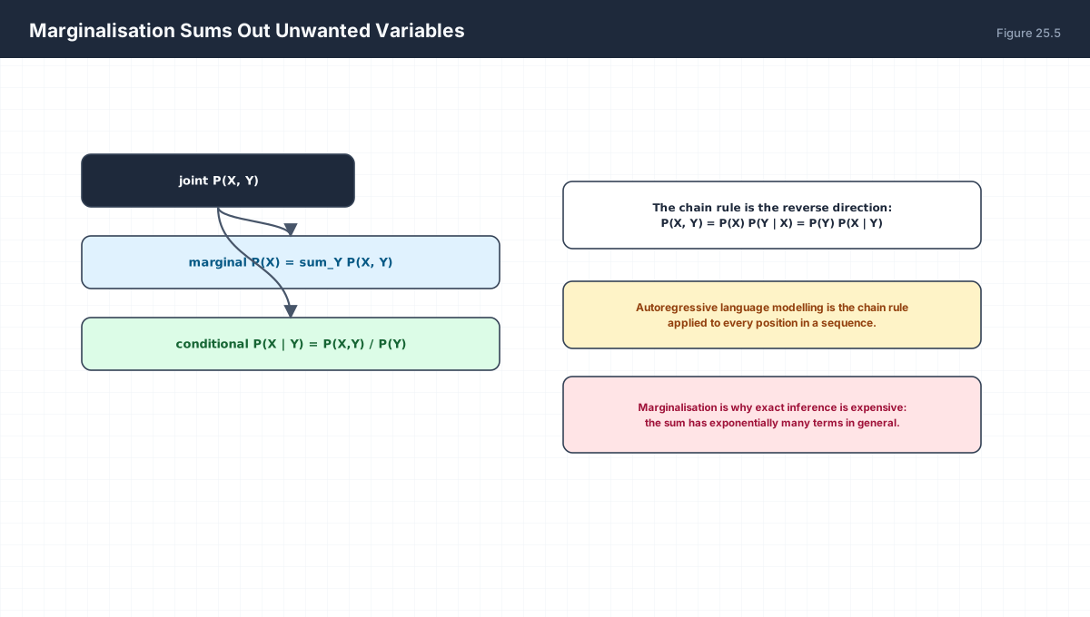
marginal      P(X) = sum_y P(X, Y = y)
conditional   P(X | Y) = P(X, Y) / P(Y)
chain rule    P(X, Y) = P(X) P(Y | X)
import numpy as np

# small joint distribution P(X, Y) as a table
joint = np.array([[0.30, 0.12],
                  [0.18, 0.40]])          # rows X=0,1   cols Y=0,1
assert np.isclose(joint.sum(), 1.0)

p_x = joint.sum(axis=1)                   # marginalise over Y
p_y = joint.sum(axis=0)
print("P(X):", p_x, " P(Y):", p_y)

p_y_given_x = joint / p_x[:, None]        # conditional per row
print("P(Y|X):\n", np.round(p_y_given_x, 4))
assert np.allclose(p_y_given_x.sum(axis=1), 1.0)

# chain rule reconstruction
rebuilt = p_x[:, None] * p_y_given_x
assert np.allclose(rebuilt, joint)
print("P(X) * P(Y|X) reconstructs the joint exactly")
Marginalisation is where exact inference becomes expensive. With n binary variables the joint has 2ⁿ entries, so summing out a subset costs exponentially many terms unless the distribution factorises. Every inference algorithm — variable elimination, belief propagation, variational methods — is a way of exploiting that factorisation.
7. Worked Examples
7.1 Complement and union
P(A) = 0.4, P(B) = 0.5, P(A and B) = 0.2
P(not A)   = 0.6
P(A or B)  = 0.4 + 0.5 - 0.2 = 0.7
7.2 Conditional from a joint
P(A and B) = 0.2, P(B) = 0.5
P(A | B) = 0.2 / 0.5 = 0.4
7.3 Testing independence
P(A) P(B) = 0.4 x 0.5 = 0.2 = P(A and B)
So in this example the events ARE independent.
Change P(A and B) to 0.1 and they are not.
7.4 Two-dice sum
36 equally likely outcomes
P(sum = 7) = 6/36 = 1/6     (1-6, 2-5, 3-4, 4-3, 5-2, 6-1)
P(sum = 2) = 1/36
7.5 Conditional dependence across a sequence
P(w1, w2, w3) = P(w1) P(w2|w1) P(w3|w1,w2)
Each factor is one model call. Independence would drop
every conditioning term and lose all context.
8. Verify It in Python
import numpy as np

rng = np.random.default_rng(0)
n = 300_000

# --- 1. axioms hold empirically -----------------------------------
dice = rng.integers(1, 7, n)
A, B = dice <= 2, dice % 2 == 0
pA, pB, pAB = A.mean(), B.mean(), (A & B).mean()
assert 0 <= pA <= 1 and 0 <= pB <= 1
assert abs((A | B).mean() - (pA + pB - pAB)) < 0.005
print("axioms and inclusion-exclusion verified")

# --- 2. complement rule -------------------------------------------
assert abs((~A).mean() + pA - 1.0) < 1e-9
print("P(A) + P(not A) = 1")

# --- 3. conditional renormalises ----------------------------------
given_B = A[B]
assert abs(given_B.mean() - pAB / pB) < 0.005
print(f"P(A|B) = {given_B.mean():.4f} matches P(A and B)/P(B) = {pAB/pB:.4f}")

# --- 4. independence test ----------------------------------------
indep_A = dice <= 3
indep_B = dice >= 4
assert abs((indep_A & indep_B).mean() - 0.0) < 1e-9      # disjoint
dep_A = dice <= 3
dep_B = dice <= 2
assert abs((dep_A & dep_B).mean() - dep_A.mean() * dep_B.mean()) > 0.01
print("dependent events fail the product test, as expected")

# --- 5. marginalisation from a joint -----------------------------
joint = np.array([[0.30, 0.12], [0.18, 0.40]])
assert np.isclose(joint.sum(), 1.0)
px, py = joint.sum(axis=1), joint.sum(axis=0)
assert np.isclose(px.sum(), 1.0) and np.isclose(py.sum(), 1.0)
print("marginals:", px, py)

# --- 6. chain rule reconstructs the joint ------------------------
cond = joint / px[:, None]
assert np.allclose(px[:, None] * cond, joint)
print("chain rule round-trips")

# --- 7. conditionals are asymmetric ------------------------------
pA_1 = joint[1].sum() / 1.0
p_cond_a = joint[1, 1] / joint[:, 1].sum()      # P(X=1 | Y=1)
p_cond_b = joint[1, 1] / joint[1, :].sum()      # P(Y=1 | X=1)
assert not np.isclose(p_cond_a, p_cond_b)
print(f"P(X=1|Y=1)={p_cond_a:.4f}  P(Y=1|X=1)={p_cond_b:.4f}")
print("all assertions passed")
9. Practice Questions
- State the three axioms and derive
P(Aᶜ) = 1 − P(A). - Given
P(A)=0.5,P(B)=0.4,P(A∩B)=0.15, computeP(A∪B). - Define
P(A|B)and explain in words what the denominator does. - Give an example where
P(A|B) ≠ P(B|A)and state both values. - State the independence condition and give two events that satisfy it.
- Why does independence not imply zero correlation in general?
- Marginalise
P(X,Y)overYgiven a 2×3 table. - Express
P(w₁,w₂,w₃)by the chain rule. - Why is exact marginalisation exponential in the number of variables?
- Explain why a language model must violate token independence.
10. Official References & Further Reading
Continue the Course
- Course Index: AI Mathematics Masterclass — All 48 Chapters
- Previous Chapter: Chapter 24: Convexity, Constraints & Lagrange Multipliers
- Next Chapter: Chapter 26: Random Variables & Probability Distributions
- Related Series: PyTorch Engineering Masterclass — All 16 Modules