
AI Reading
Quick summary of this article
AI Mathematics Masterclass — Chapter 27 of 48
Expectation, variance and covariance are the three numbers that summarise a distribution, and each maps directly onto something in a training run. Expectation is the loss you are minimising. Variance is the noise you are fighting and the bias–variance trade-off you are navigating. Covariance is the structure that PCA exploits and that correlated features break.
1. Technical Audit & Core Learning Objectives
| Component | Common Tutorial Deficiency | Engineering Standard Applied Here |
|---|---|---|
| Expectation | Treated as “the average” with no note on linearity. | Linearity stated as the property that makes batching valid. |
| Variance | Formula given twice without connecting them. | Both forms shown, with the one-pass version used in code. |
| Covariance | Defined but not extended to the matrix. | Covariance matrix linked forward to PCA in Chapter 36. |
| Decomposition | Bias–variance quoted as a slogan. | Derived, with the noise term shown as irreducible. |
Core learning objectives. After this chapter you should be able to:
- Compute
E[X]for a discrete distribution and state linearity. - Compute
Var(X)from either definition and explain the shortcut. - Compute covariance and interpret its sign.
- Derive
Var(X+Y)and explain the role of covariance. - Relate the standard error to sample count.
- State the bias–variance decomposition and identify the irreducible term.
2. Expectation
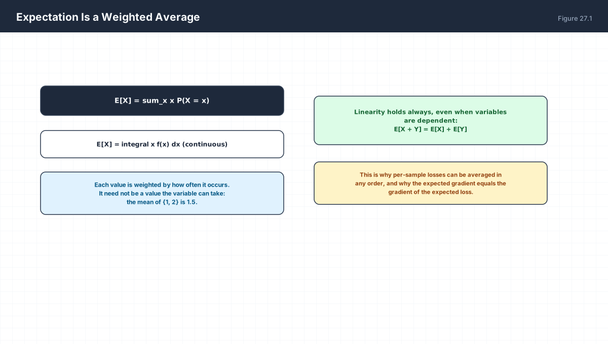
discrete      E[X] = sum_x x p(x)
continuous    E[X] = integral x f(x) dx

linearity     E[aX + b] = aE[X] + b
              E[X + Y] = E[X] + E[Y]      always, even if dependent
import numpy as np

rng = np.random.default_rng(0)

# discrete: a loaded die
faces = np.array([1, 2, 3, 4, 5, 6])
probs = np.array([0.1, 0.1, 0.1, 0.2, 0.2, 0.3])
E = (faces * probs).sum()
print(f"E[X] = {E:.4f}")
assert np.isclose(probs.sum(), 1.0)

samples = rng.choice(faces, size=500_000, p=probs)
print(f"empirical mean {samples.mean():.4f}")

# linearity with dependent variables
X = rng.normal(0, 1, 200_000)
Y = 2 * X + rng.normal(0, 0.1, 200_000)         # strongly dependent
print(f"E[X+Y]={np.mean(X+Y):.4f}  E[X]+E[Y]={X.mean()+Y.mean():.4f}")
assert abs(np.mean(X + Y) - (X.mean() + Y.mean())) < 0.01
3. Variance
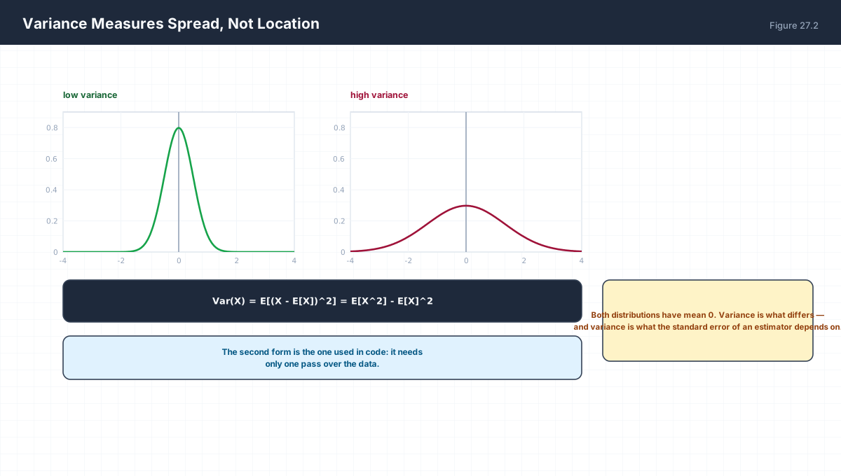
Var(X) = E[(X - E[X])^2]        definition
       = E[X^2] - E[X]^2        one-pass form, used in code
SD(X)  = sqrt(Var(X))           same units as X
import numpy as np

rng = np.random.default_rng(1)
X = rng.normal(3.0, 2.0, 300_000)

two_pass = np.mean((X - X.mean()) ** 2)
one_pass = np.mean(X ** 2) - X.mean() ** 2
print(f"two-pass {two_pass:.4f}   one-pass {one_pass:.4f}   (expect 4.0)")
assert abs(two_pass - one_pass) < 1e-6

# variance scales quadratically
print("Var(2X) =", round(np.var(2 * X), 3), " 4*Var(X) =", round(4 * np.var(X), 3))
assert np.isclose(np.var(2 * X), 4 * np.var(X))
The one-pass form is faster but numerically worse for large means: E[X²] and E[X]² can be nearly equal and huge, so their difference loses precision. NumPy uses a compensated algorithm; a hand-rolled loop over values near 1e9 will not.
4. Covariance
import numpy as np

rng = np.random.default_rng(2)
X = rng.normal(0, 1, 100_000)

pos = 2 * X + rng.normal(0, 0.3, X.size)
neg = -1.5 * X + rng.normal(0, 0.3, X.size)
unc = rng.normal(0, 1, X.size)

for name, Y in (("positive", pos), ("negative", neg), ("independent", unc)):
    cov = np.cov(X, Y)[0, 1]
    print(f"{name:12s} cov = {cov:+.4f}")

# the covariance matrix of a stack
data = np.vstack([X, pos, neg])
C = np.cov(data)
print("\ncovariance matrix shape:", C.shape)
print(np.round(C, 3))
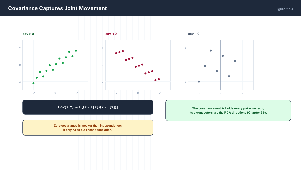
Note that zero covariance does not imply independence. The classic counterexample is X ~ N(0,1) with Y = X²: they are perfectly dependent, yet Cov(X,Y) = 0 because the relationship is symmetric and non-linear. Covariance only measures linear association.
5. Variance of a Sum, and Standard Error
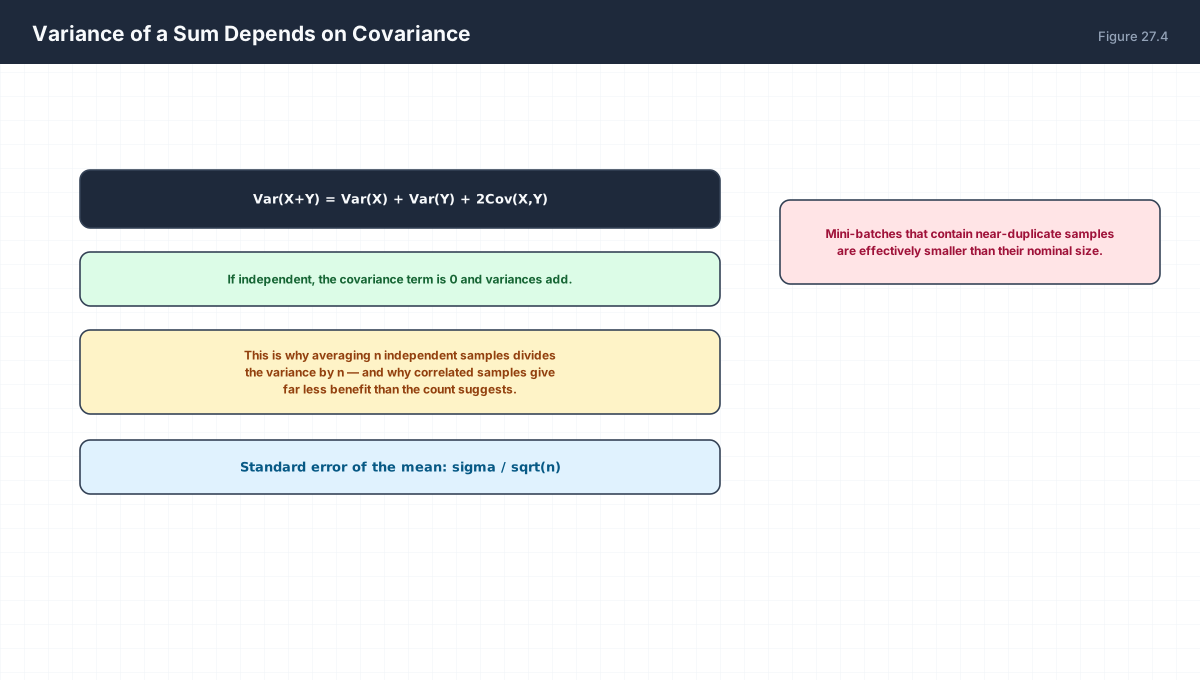
Var(X + Y) = Var(X) + Var(Y) + 2 Cov(X, Y)

Independent:  Var(X + Y) = Var(X) + Var(Y)
Mean of n:    Var(Xbar) = Var(X) / n      ->  SE = sigma / sqrt(n)
import numpy as np

rng = np.random.default_rng(3)

# independent
X = rng.normal(0, 1, 200_000)
Y = rng.normal(0, 1, 200_000)
print(f"independent: Var(X+Y)={np.var(X+Y):.4f}  sum of vars={np.var(X)+np.var(Y):.4f}")

# perfectly correlated
Z = X.copy()
print(f"identical  : Var(X+Z)={np.var(X+Z):.4f}  sum of vars={np.var(X)+np.var(Z):.4f}")

# standard error
for n in (100, 1000, 10000):
    means = rng.normal(0, 1, size=(4000, n)).mean(axis=1)
    print(f"n={n:6d}  SE observed {means.std():.4f}  predicted {1/np.sqrt(n):.4f}")
6. Bias–Variance Decomposition
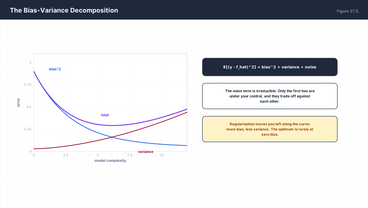
E[(y - f_hat(x))^2] = bias(f_hat)^2 + Var(f_hat) + sigma^2
                       ^model too simple  ^model too complex  ^noise
| Term | Cause | Reduced By |
|---|---|---|
| Bias | Model too constrained | More capacity |
| Variance | Sensitivity to the training sample | Regularisation, more data, ensembling |
| Noise | Irreducible randomness in the data | Nothing |
The decomposition is why more capacity is not always better, and why an ensemble of high-variance models beats any single member: averaging reduces variance by roughly 1/n while leaving bias untouched.
7. Worked Examples
7.1 Loaded die
p = [0.1,0.1,0.1,0.2,0.2,0.3] on faces 1..6
E[X]   = 4.2
E[X^2] = 20.4
Var    = 20.4 - 17.64 = 2.76
7.2 Scaling and shifting
Var(aX + b) = a^2 Var(X)
Var(3X + 7) = 9 Var(X)
The shift does not affect spread; the scale affects it quadratically.
7.3 Standard error
sigma = 2, n = 100  ->  SE = 0.2
To get SE = 0.1 you need n = 400, not 200.
7.4 Covariance of a sum, twice
Var(X + Y) with Cov = 0.5, Var(X) = Var(Y) = 1
= 1 + 1 + 2(0.5) = 3
Twice what independence would give.
7.5 Correlation
Corr(X,Y) = Cov(X,Y) / (SD(X) SD(Y))
Always in [-1, 1]. Scale-free, unlike covariance.
8. Verify It in Python
import numpy as np

rng = np.random.default_rng(0)

# --- 1. expectation of a discrete variable ------------------------
faces, probs = np.array([1, 2, 3, 4, 5, 6]), np.array([.1, .1, .1, .2, .2, .3])
E = (faces * probs).sum()
assert np.isclose(E, 4.2)
print("E[X] =", E)

# --- 2. variance both ways ---------------------------------------
var_def = ((faces - E) ** 2 * probs).sum()
var_short = (faces ** 2 * probs).sum() - E ** 2
assert np.isclose(var_def, var_short)
print("Var =", round(var_def, 4))

# --- 3. linearity with dependence --------------------------------
X = rng.normal(0, 1, 200_000)
Y = 3 * X + rng.normal(0, .5, X.size)
assert abs((X + Y).mean() - (X.mean() + Y.mean())) < 0.01
print("E[X+Y] == E[X]+E[Y] despite dependence")

# --- 4. variance of a sum needs covariance -----------------------
bare = np.var(X) + np.var(Y)
full = bare + 2 * np.cov(X, Y)[0, 1]
assert np.isclose(np.var(X + Y), full, rtol=0.02)
assert not np.isclose(np.var(X + Y), bare, rtol=0.02)
print(f"Var(X+Y)={np.var(X+Y):.4f}  naive={bare:.4f}  with cov={full:.4f}")

# --- 5. zero covariance does not mean independence ---------------
Z = rng.normal(0, 1, 200_000)
assert abs(np.cov(Z, Z ** 2)[0, 1]) < 0.05       # covariance ~ 0
assert not np.allclose(np.sort(Z), np.sort(np.abs(Z)))   # clearly dependent
print("Cov(X, X^2) ~ 0 even though X and X^2 are dependent")

# --- 6. correlation is bounded -----------------------------------
for scale in (1, 1000):
    c = np.corrcoef(X, scale * X + rng.normal(0, .1, X.size))[0, 1]
    assert -1.0001 <= c <= 1.0001
print("correlation stays in [-1, 1]")

# --- 7. standard error scales as 1/sqrt(n) ----------------------
ses = {}
for n in (100, 1600):
    ses[n] = rng.normal(0, 1, size=(3000, n)).mean(axis=1).std()
assert abs(ses[1600] / ses[100] - 0.25) < 0.03      # sqrt(100/1600) = 0.25
print("SE ratio for 16x data:", round(ses[1600] / ses[100], 4), "(expect 0.25)")

# --- 8. averaging reduces variance ------------------------------
single = rng.normal(0, 1, size=(4000, 1))
many = rng.normal(0, 1, size=(4000, 50))
assert many.mean(axis=1).var() < single.mean(axis=1).var()
print("ensemble variance < single-model variance")
print("all assertions passed")
9. Practice Questions
- Compute
E[X]andVar(X)for a fair die. - State the linearity of expectation and why it needs no independence.
- Prove
Var(X) = E[X²] − E[X]². - Compute
Var(4X + 10)givenVar(X) = 3. - Give two dependent variables with zero covariance.
- Derive
Var(X + Y)including the covariance term. - If
σ = 5, whatngives a standard error of 0.25? - State the bias–variance decomposition and label the irreducible term.
- Why does ensembling reduce variance but not bias?
- Why is correlation preferred to covariance when comparing across scales?
10. Official References & Further Reading
Continue the Course
- Course Index: AI Mathematics Masterclass — All 48 Chapters
- Previous Chapter: Chapter 26: Random Variables & Probability Distributions
- Next Chapter: Chapter 28: Bayes' Theorem & Bayesian Inference
- Related Series: PyTorch Engineering Masterclass — All 16 Modules