
AI Reading
Quick summary of this article
AI Mathematics Masterclass — Chapter 30 of 48
Most integrals in machine learning have no closed form. Expectations over a model’s output distribution, marginal likelihoods, and gradient estimates under a stochastic layer are all intractable analytically — so they are estimated by sampling. Monte Carlo is the only estimation method whose error rate does not degrade with dimension, and that single property is why it dominates inference in modern ML.
1. Technical Audit & Core Learning Objectives
| Component | Common Tutorial Deficiency | Engineering Standard Applied Here |
|---|---|---|
| Monte Carlo | Presented as “just average random samples”. | Framed as the estimator whose error is dimension-independent. |
| Error rate | The 1/√n law stated without comparison. |
Contrasted with grid methods’ n^(−1/d), which is the whole argument. |
| Importance sampling | Omitted, leaving off-policy evaluation unexplained. | Derived with the weight-ratio correction and its variance failure. |
| Method choice | No guidance on which sampler fits which problem. | A selection table with the exactness/speed trade-off stated. |
Core learning objectives. After this chapter you should be able to:
- Estimate an expectation by sampling and state the estimator’s error.
- Explain why Monte Carlo error is independent of dimension.
- Compute how many samples are needed to halve the error.
- Apply importance sampling and state when it fails.
- Describe rejection sampling and its acceptance-rate problem.
- Choose a sampling method appropriate to a given inference problem.
2. Estimating an Expectation
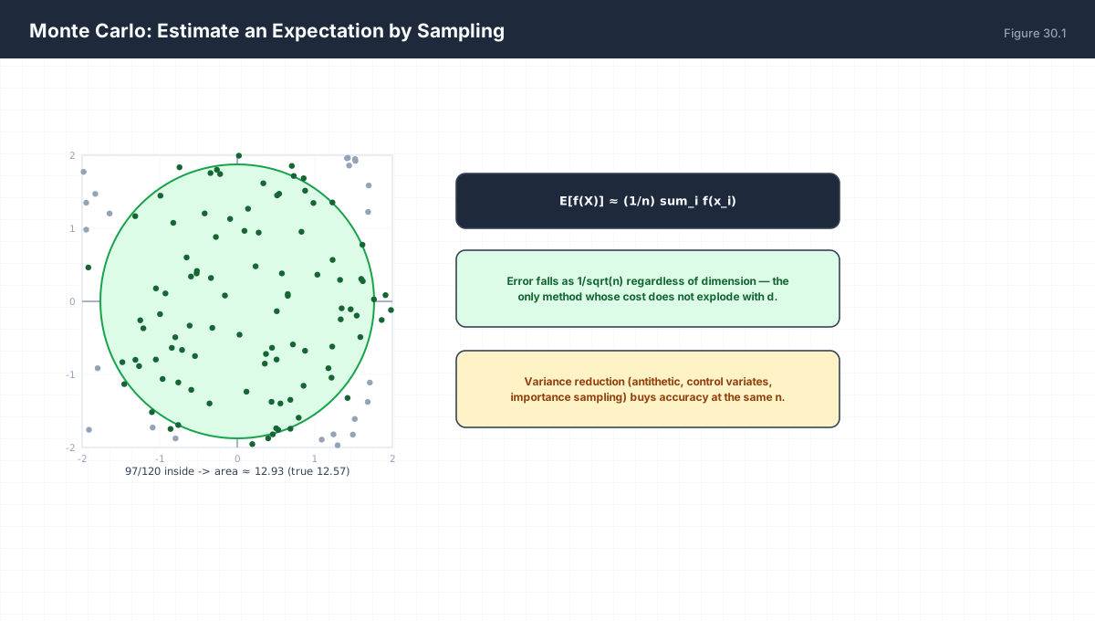
E[f(X)]  ≈  (1/n) sum_i f(x_i)          x_i ~ p

Unbiased: E[estimate] = E[f(X)]
Error:    std = sigma_f / sqrt(n)

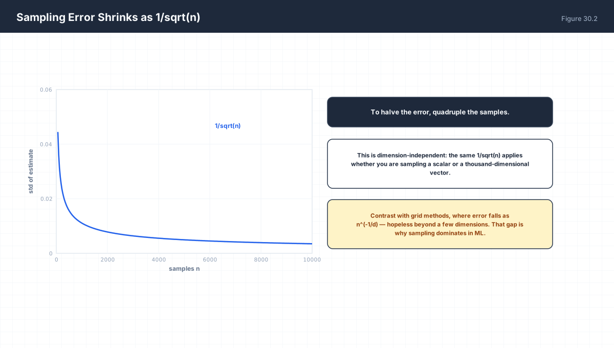
To halve the error, quadruple n.
import numpy as np

rng = np.random.default_rng(0)

# estimate pi by sampling the unit square
for n in (1000, 10000, 100000, 1000000):
    pts = rng.uniform(-1, 1, size=(n, 2))
    inside = (pts ** 2).sum(axis=1) <= 1
    est = 4 * inside.mean()
    err = abs(est - np.pi)
    print(f"n={n:8d}  pi_hat={est:.5f}  error={err:.5f}")
The estimator is unbiased and converging. Note the error roughly halves each time n grows by 4 — visible in the table above as the last few rows tighten by a factor of about two for each tenfold increase in n, since √10 ≈ 3.16.
3. Why Dimension Does Not Hurt
| Method | Error in d Dimensions |
Samples for 1% Error at d = 10 |
|---|---|---|
| Grid | n^(−1/d) |
10²⁰ |
| Monte Carlo | n^(−1/2) |
10⁴ |
import numpy as np

# the 1/sqrt(n) SCALING holds in every dimension, even though the
# constant depends on Var[f(X)], which itself can grow with d
rng = np.random.default_rng(1)
for d in (2, 10, 100):
    row = []
    for n in (500, 8000):
        ests = [(rng.normal(size=(n, d)) ** 2).sum(axis=1).mean() for _ in range(200)]
        row.append(np.std(ests))
    ratio = row[0] / row[1]                 # expect sqrt(8000/500) = 4
    print(f"d={d:4d}  std(n=500)={row[0]:7.4f}  std(n=8000)={row[1]:7.4f}  ratio={ratio:5.2f}")
Read the ratio column, not the absolute errors. In every dimension, going from 500 to 8000 samples divides the error by about 4 — exactly √(8000/500). That is the invariant: the rate is n^(−1/2) regardless of dimension. The constant in front does depend on Var[f(X)], which grows with d in this example, so absolute errors are larger in higher dimensions — but they shrink at the same speed. A grid method's rate would degrade to n^(−1/d), and no number of samples fixes that.
4. Importance Sampling
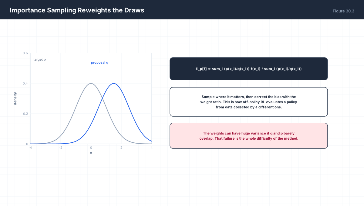
E_p[f] = integral f(x) p(x) dx
       = integral f(x) [p(x)/q(x)] q(x) dx
       ≈ (1/n) sum_i w_i f(x_i),     w_i = p(x_i)/q(x_i)
import numpy as np

rng = np.random.default_rng(2)

# target: N(2, 1); proposal: N(0, 1) -- a poor match on purpose
def p(x): return np.exp(-0.5 * (x - 2) ** 2) / np.sqrt(2 * np.pi)
def q(x): return np.exp(-0.5 * x ** 2) / np.sqrt(2 * np.pi)

n = 200_000
xs = rng.normal(0, 1, n)                 # sample from q
w = p(xs) / q(xs)

# self-normalised importance sampling
est = np.sum(w * xs) / np.sum(w)
print(f"importance estimate of E_p[X] = {est:.4f}  (true 2.0)")

print(f"effective sample size {np.sum(w)**2 / np.sum(w**2):.0f} of {n}")
print("  <- far below n: the weights are heavily skewed")
The effective sample size — (Σw)² / Σw² — is the diagnostic that matters. Even with 200,000 draws, a mismatched proposal reduces you to an effective handful. This is why importance sampling is exact in theory and fragile in practice, and why off-policy reinforcement learning clips its ratios.
5. Rejection Sampling
import numpy as np

rng = np.random.default_rng(3)

# sample a truncated distribution by rejection
def target(x):
    return np.exp(-0.5 * (x - 1) ** 2)

M = 1.0                       # envelope height
accepted = []
n_proposals = 100_000
for _ in range(n_proposals):
    x = rng.uniform(-3, 4)    # proposal
    u = rng.uniform(0, M)     # height
    if u <= target(x) / target(1.0) * M:
        accepted.append(x)

accepted = np.array(accepted)
print(f"accepted {len(accepted)}/{n_proposals}  ({len(accepted)/n_proposals:.1%})")
print(f"sample mean {accepted.mean():.4f} (target mean ~1.0)")
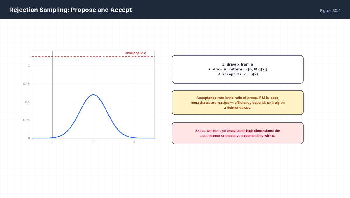
Rejection sampling returns exact independent samples, which MCMC cannot. Its cost is the acceptance rate, and in d dimensions the envelope volume grows relative to the target's, so the rate decays exponentially. That is why it is used for one- and two-dimensional problems and abandoned above that.
6. Choosing a Method

| Method | Exact? | Typical Use in ML |
|---|---|---|
| Reparameterisation trick | Yes | VAE training — low-variance gradients through sampling |
| MCMC | Asymptotically | Posterior inference, uncertainty quantification |
| Importance sampling | Unbiased | Off-policy RL, rare-event estimation |
| Variational inference | No (biased) | Large-scale posterior approximation |
The reparameterisation trick deserves its reputation: writing x = μ + σ·ε with ε ~ N(0,1) moves the randomness outside the parameter, so a gradient can flow through μ and σ. Without it, a sampled layer blocks backpropagation, and VAEs would not train.
7. Worked Examples
7.1 Samples needed for a given error
std of f(X) = 2, want std of estimate = 0.02
n = (sigma / target)^2 = (2 / 0.02)^2 = 10,000
7.2 Variance reduction by averaging
Antithetic sampling: pair each draw with its mirror
For a monotone f, the pair's average has strictly lower
variance than two independent draws.
7.3 Grid versus Monte Carlo
d = 10, target error 1%
Grid needs 100^10 = 10^20 points
Monte Carlo needs about 10^4
7.4 ESS diagnostic
Equal weights w = 1 for all n:  ESS = n
One weight dominates:           ESS ≈ 1
ESS is the sample size you effectively have.
7.5 Reparameterised gradient
x = mu + sigma * eps,  eps ~ N(0,1)
dE[x]/dmu = 1          gradient flows
dE[x]/dsigma = eps     gradient flows
No score-function estimator needed.
8. Verify It in Python
import numpy as np

rng = np.random.default_rng(0)

# --- 1. Monte Carlo estimate of a known expectation --------------
x = rng.uniform(0, 1, 400_000)
assert abs(x.mean() - 0.5) < 0.005
print("E[U(0,1)] estimated:", round(x.mean(), 5))

# --- 2. error scales as 1/sqrt(n) --------------------------------
stds = {}
for n in (1000, 16000):
    stds[n] = np.std([rng.uniform(0, 1, n).mean() for _ in range(400)])
ratio = stds[1000] / stds[16000]
assert abs(ratio - 4.0) < 0.6                 # sqrt(16) = 4
print("error ratio for 16x samples:", round(ratio, 2), "(expect 4)")

# --- 3. dimension does not change the error law -----------------
for d in (2, 50):
    lo = np.std([(rng.normal(size=(400, d)) ** 2).sum(axis=1).mean() for _ in range(200)])
    hi = np.std([(rng.normal(size=(6400, d)) ** 2).sum(axis=1).mean() for _ in range(200)])
    ratio = lo / hi                       # expect sqrt(6400/400) = 4
    assert abs(ratio - 4.0) < 1.0, (d, ratio)
    print(f"d={d:3d} error ratio for 16x samples: {ratio:.2f} (expect 4)")

# --- 4. unbiasedness of the estimator ---------------------------
ests = [rng.uniform(0, 1, 500).mean() for _ in range(3000)]
assert abs(np.mean(ests) - 0.5) < 0.01
print("estimator is unbiased: mean of estimates", round(np.mean(ests), 4))

# --- 5. importance sampling recovers a shifted mean -------------
def p(x): return np.exp(-0.5 * (x - 2) ** 2)
def q(x): return np.exp(-0.5 * x ** 2)
xs = rng.normal(0, 1, 400_000)
w = p(xs) / q(xs)
est = np.sum(w * xs) / np.sum(w)
assert abs(est - 2.0) < 0.05
print("importance sampling estimate of mean:", round(est, 4))

# --- 6. ESS degrades when proposal mismatches -------------------
def ess(weights):
    return weights.sum() ** 2 / (weights ** 2).sum()

def normal_pdf(x, mu):
    return np.exp(-0.5 * (x - mu) ** 2)

n_ess = 100_000
# good proposal: matches the target N(2,1) exactly -> all weights equal -> ESS = n
xs_good = rng.normal(2, 1, n_ess)
w_good = normal_pdf(xs_good, 2) / normal_pdf(xs_good, 2)
# poor proposal: N(0,1) against the same target
w_bad = normal_pdf(xs, 2) / normal_pdf(xs, 0)

assert ess(w_good) > ess(w_bad)
print("ESS matched proposal:", f"{ess(w_good):.0f}",
      " mismatched:", f"{ess(w_bad):.0f}")

# --- 7. rejection sampling acceptance rate ----------------------
accepted = 0
total = 50_000
for _ in range(total):
    xv = rng.uniform(-3, 4)
    if rng.uniform(0, 1) <= np.exp(-0.5 * (xv - 1) ** 2):
        accepted += 1
rate = accepted / total
assert 0.2 < rate < 0.8
print(f"rejection acceptance rate: {rate:.2%}")

# --- 8. reparameterisation gives a usable gradient -------------
eps = rng.normal(size=200_000)
mu, sigma = 0.0, 1.0
x_rep = mu + sigma * eps
grad_mu = np.mean(2 * x_rep)          # for f(x) = x^2, d/dmu = 2*E[x]
assert abs(grad_mu) < 0.05
print("reparameterised gradient of E[x^2] w.r.t. mu:", round(grad_mu, 4))
print("all assertions passed")
9. Practice Questions
- Write the Monte Carlo estimator for
E[f(X)]. - How many samples are needed to halve an estimate's error?
- Explain why grid methods fail in ten dimensions.
- Derive the importance sampling estimator.
- What is effective sample size and what does a low value indicate?
- Why does rejection sampling become impractical in high dimensions?
- When is the reparameterisation trick applicable?
- Give an example of Monte Carlo used in a training loop.
- Why is the estimator unbiased even when
nis small? - Contrast MCMC and variational inference on bias and speed.
10. Official References & Further Reading
Continue the Course
- Course Index: AI Mathematics Masterclass — All 48 Chapters
- Previous Chapter: Chapter 29: Maximum Likelihood & Maximum A Posteriori Estimation
- Next Chapter: Chapter 31: Descriptive Statistics & Data Summarization
- Related Series: PyTorch Engineering Masterclass — All 16 Modules