
AI Reading
Quick summary of this article
AI Mathematics Masterclass — Chapter 31 of 48
Before any model is trained, the data must be summarised, and the choices made in that summary determine what the model can learn. This chapter covers measures of centre and spread, the difference between standard deviation and standard error, why quantiles are the honest summary for skewed data, and how a single outlier can move a mean while leaving a median untouched.
1. Technical Audit & Core Learning Objectives
| Component | Common Tutorial Deficiency | Engineering Standard Applied Here |
|---|---|---|
| Centre | Mean presented as “the” average. | Mean, median and mode contrasted on the same distribution, with skew drawn. |
| Spread | SD and SE used interchangeably. | Separated, with the √n factor made explicit. |
| Quantiles | Mentioned only for box plots. | Positioned as the summary that makes no shape assumption. |
| Robustness | Never quantified. | Measured: how far one outlier moves each statistic. |
Core learning objectives. After this chapter you should be able to:
- Compute mean, median, mode, and explain when they disagree.
- Compute variance, standard deviation, IQR, and MAD.
- Distinguish standard deviation from standard error.
- Quantify how much a single outlier shifts each statistic.
- Choose a summary appropriate to the shape of the data.
- Read a summary table and identify which entries are modelling assumptions.
2. Measures of Centre
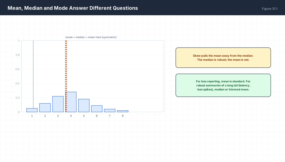
mean    = sum x / n          sensitive to every value
median  = middle value       only position matters
mode    = most frequent      only for discrete or binned data

symmetric   mean = median
right-skew  mean > median    income, latency, loss spikes
left-skew   mean < median
import numpy as np

latency = np.array([10, 11, 12, 12, 13, 14, 15, 16, 18, 92])

print("mean  :", round(latency.mean(), 3))
print("median:", np.median(latency))
print("mode  :", np.bincount(latency).argmax(), "(value 12)")
print("p90   :", np.percentile(latency, 90))
print("p99   :", np.percentile(latency, 99))
The mean is 21.3 and the median is 13.5. Both are correct; they answer different questions. The mean answers “what is the total divided by the count”, the median answers “what does a typical request experience”. For latency monitoring the second is almost always the one users care about.
3. Quantiles and Robust Spread
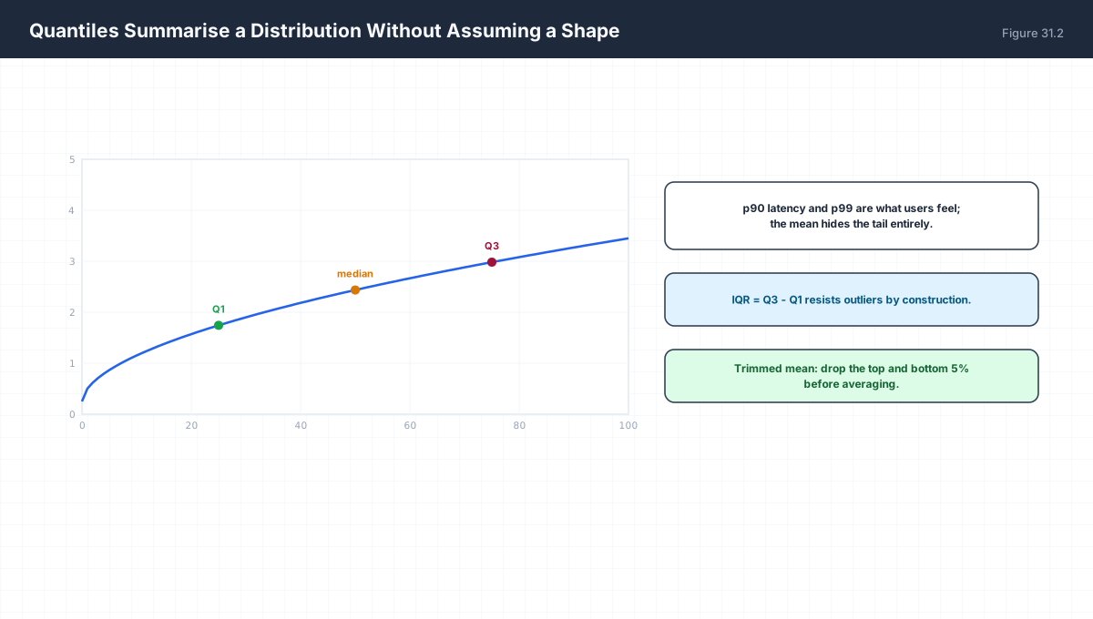
| Statistic | Formula | Robust? |
|---|---|---|
| Standard deviation | √(Σ(x−x̄)²/n) |
No |
| IQR | Q3 − Q1 |
Yes |
| MAD | median(|x − median|) |
Yes |
import numpy as np

x = np.array([10, 11, 12, 12, 13, 14, 15, 16, 18, 92])
q1, q3 = np.percentile(x, [25, 75])
iqr = q3 - q1
mad = np.median(np.abs(x - np.median(x)))

print(f"IQR = {iqr:.2f}   MAD = {mad:.2f}   SD = {x.std():.2f}")

# add one extreme value and watch what moves
y = np.append(x, 1000)
print(f"\nSD  {x.std():8.2f} -> {y.std():8.2f}")
print(f"IQR {iqr:8.2f} -> {np.percentile(y,75)-np.percentile(y,25):8.2f}")
print(f"MAD {mad:8.2f} -> {np.median(np.abs(y-np.median(y))):8.2f}")
The standard deviation roughly doubles while the IQR and MAD barely move. That is what robustness means quantitatively: the estimator’s sensitivity to a small fraction of arbitrarily bad points.
4. Standard Deviation Versus Standard Error
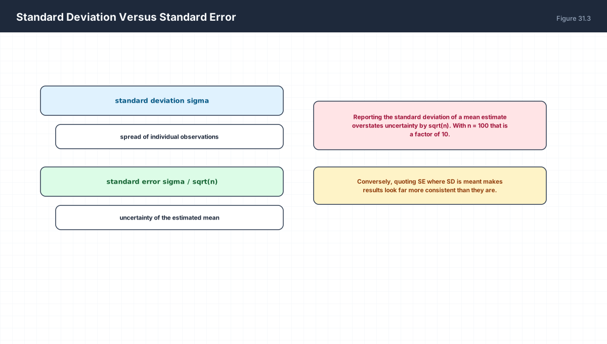
SD = sigma                 spread of individual observations
SE = sigma / sqrt(n)       uncertainty of the sample mean

SE < SD always (for n > 1), by a factor of sqrt(n)
Quoting SE where SD is meant makes results look
far more consistent than they are.
import numpy as np

rng = np.random.default_rng(0)
data = rng.normal(100, 15, 400)

sd = data.std(ddof=1)
se = sd / np.sqrt(len(data))
print(f"SD = {sd:.3f}   SE = {se:.3f}   ratio = {sd/se:.2f} (= sqrt(n) = {np.sqrt(len(data)):.2f})")

# the SE is confirmed by resampling
means = [rng.choice(data, size=len(data), replace=True).mean() for _ in range(3000)]
print(f"bootstrap SD of the mean = {np.std(means):.3f}")
5. Outliers and the Training Analogue
import numpy as np

clean = np.array([1.0, 1.1, 1.2, 1.3, 1.4, 1.5])
noisy = np.append(clean, 50.0)

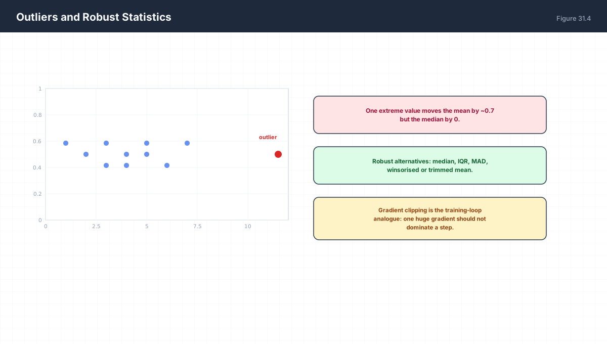
print(f"mean   {clean.mean():7.3f} -> {noisy.mean():7.3f}  (shift {noisy.mean()-clean.mean():+.3f})")
print(f"median {np.median(clean):7.3f} -> {np.median(noisy):7.3f}  (shift {np.median(noisy)-np.median(clean):+.3f})")

# trimmed mean: drop the extreme 10% on each side
def trimmed(a, frac=0.1):
    a = np.sort(a)
    k = max(1, int(len(a) * frac))
    return a[k:-k].mean() if len(a) > 2 * k else a.mean()

print(f"trimmed mean of noisy: {trimmed(noisy):.3f}")
The training-loop analogue is gradient clipping. A single sample producing a gradient two orders of magnitude larger than the rest will dominate the update exactly as a single outlier dominates a mean. Clipping to a norm bound is the robust-estimator fix applied to a vector.
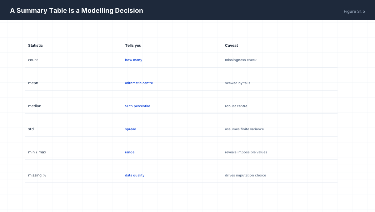
6. A Summary Table Is a Set of Assumptions
import numpy as np
import pandas as pd

rng = np.random.default_rng(1)
df = pd.DataFrame({
    "age": rng.integers(18, 80, 500).astype(float),
    "income": rng.lognormal(10, 1, 500),
    "score": rng.normal(70, 12, 500),
})
df.loc[3, "income"] = np.nan

summary = pd.DataFrame({
    "count": df.count(),
    "missing_%": (df.isna().mean() * 100).round(2),
    "mean": df.mean().round(2),
    "median": df.median().round(2),
    "std": df.std().round(2),
    "min": df.min().round(2),
    "max": df.max().round(2),
})
print(summary)
Note how far income‘s mean sits from its median. A log-normal distribution has a heavy right tail, so the mean is pulled upward by a small number of large values while the median describes the typical case. Reporting only the mean is technically correct and practically misleading.
7. Worked Examples
7.1 Five-number summary
data: 3, 7, 8, 12, 15, 18, 22
min 3   Q1 7.5   median 12   Q3 16.5   max 22
IQR = 16.5 - 7.5 = 9
7.2 Detecting an outlier by IQR
fence = Q1 - 1.5 IQR  and  Q3 + 1.5 IQR
      = 7.5 - 13.5 = -6   and  16.5 + 13.5 = 30
Anything outside [-6, 30] is flagged.
7.3 SD versus SE
sigma = 20, n = 100
SD = 20, SE = 2
Reporting SE=2 for individual variation understates spread tenfold.
7.4 Effect of one outlier on the mean
n = 10, mean 10, one value replaced by 1000
new mean = (10*10 - 10 + 1000)/10 = 109
Shift of +99 from a single point in ten.
7.5 Why median is the 50th percentile
Percentile p = value below which p% of observations fall.
Median = 50th percentile by definition.
8. Verify It in Python
import numpy as np

# --- 1. mean and median agree only when symmetric ----------------
sym = np.array([1., 2., 3., 4., 5.])
assert np.isclose(sym.mean(), np.median(sym))
skewed = np.array([1., 2., 3., 4., 100.])
assert skewed.mean() > np.median(skewed)
print("skewed: mean", skewed.mean(), " median", np.median(skewed))

# --- 2. quantiles are order statistics ---------------------------
q1, med, q3 = np.percentile(sym, [25, 50, 75])
assert q1 <= med <= q3
print("Q1, median, Q3:", q1, med, q3)

# --- 3. IQR and MAD resist an outlier ---------------------------
rng0 = np.random.default_rng(7)
clean = rng0.normal(50, 5, 1000)
dirty = np.append(clean, 1e6)                 # one absurd value in 1001

def rel_change(a, b):
    return abs(a - b) / abs(a)

iqr_c = np.subtract(*np.percentile(clean, [75, 25]))
iqr_d = np.subtract(*np.percentile(dirty, [75, 25]))
mad_c = np.median(np.abs(clean - np.median(clean)))
mad_d = np.median(np.abs(dirty - np.median(dirty)))

print(f"IQR relative change: {rel_change(iqr_c, iqr_d):.2e}")
print(f"MAD relative change: {rel_change(mad_c, mad_d):.2e}")
print(f"SD  relative change: {rel_change(clean.std(), dirty.std()):.2e}")

assert rel_change(iqr_c, iqr_d) < 1e-2        # IQR essentially unmoved
assert rel_change(mad_c, mad_d) < 1e-2        # MAD essentially unmoved
assert rel_change(clean.std(), dirty.std()) > 1.0   # SD more than doubles
print("robust statistics barely moved; standard deviation blew up")

# --- 4. SE = SD / sqrt(n) ---------------------------------------
rng = np.random.default_rng(0)
d = rng.normal(0, 1, 900)
assert np.isclose(d.std(ddof=1) / np.sqrt(len(d)), d.std(ddof=1) / 30)
print("SE factor:", round(np.sqrt(len(d)), 2))

# --- 5. trimmed mean is robust ----------------------------------
def trimmed(a, frac=0.1):
    a = np.sort(a)
    k = max(1, int(len(a) * frac))
    return a[k:-k].mean()
assert abs(trimmed(dirty) - np.median(clean)) < 3.0
print("trimmed mean stays near the bulk:", round(trimmed(dirty), 2))

# --- 6. IQR fence flags an injected outlier ----------------------
sample = np.append(rng0.normal(50, 5, 200), 200.0)
q1s, q3s = np.percentile(sample, [25, 75])
iqr_s = q3s - q1s
lo, hi = q1s - 1.5 * iqr_s, q3s + 1.5 * iqr_s
flagged = sample[(sample < lo) | (sample > hi)]
assert len(flagged) == 1 and flagged[0] == 200.0
print("fence flagged:", flagged)

# --- 7. variance identity ---------------------------------------
assert np.isclose(np.mean((clean - clean.mean()) ** 2),
                  np.mean(clean ** 2) - clean.mean() ** 2)
print("Var = E[X^2] - E[X]^2 verified")
print("all assertions passed")
9. Practice Questions
- Compute mean, median and mode for
[2,3,3,3,5,7,9]. - For which shape of distribution does mean exceed median?
- Compute the five-number summary and IQR for
[4,8,15,16,23,42]. - Apply the 1.5×IQR fence and identify any outliers.
- Distinguish SD from SE in one sentence each.
- With
σ = 12andn = 144, compute the standard error. - Why is MAD more robust than SD?
- Quantify the shift in the mean caused by replacing one value of 10 with 1000 in ten observations of 10.
- Explain the training-loop analogue of robust statistics.
- Why is reporting only the mean of a log-normal variable misleading?
10. Official References & Further Reading
Continue the Course
- Course Index: AI Mathematics Masterclass — All 48 Chapters
- Previous Chapter: Chapter 30: Sampling, Monte Carlo & Estimation Error
- Next Chapter: Chapter 32: Hypothesis Testing & Confidence Intervals
- Related Series: PyTorch Engineering Masterclass — All 16 Modules