
AI Reading
Quick summary of this article
AI Mathematics Masterclass — Chapter 4 of 48
Exponentiation and its inverse, the logarithm, are the two operations that connect probability to arithmetic in machine learning. Softmax exponentiates logits so they become positive; cross-entropy takes logarithms so that multiplication becomes addition; perplexity exponentiates back so the number is interpretable. This chapter builds the algebra, then uses it to explain two things that break in practice: why a log scale is mandatory for loss curves, and why naive exp silently returns inf or 0.0 on perfectly ordinary inputs.
1. Technical Audit & Core Learning Objectives
Most expositions present exponent rules as algebra to memorise and logarithms as a calculator button. Neither explains why every language model reports its quality in perplexity, or why a softmax implementation without max-subtraction fails on inputs that are mathematically unremarkable.
| Component | Common Tutorial Deficiency | Engineering Standard Applied Here |
|---|---|---|
| Exponent laws | Rules stated, then abandoned; never used again. | Every rule connected to a transformation actually performed in softmax and log-space arithmetic. |
| Log scale | Treated as a plotting preference. | Shown to be the correct scale whenever the quantity is a ratio — loss, perplexity, learning rate. |
| Softmax | Presented as a formula, with no numerical discussion. | Derived, then hardened with max-subtraction; the failure it prevents is demonstrated. |
| Information | Cross-entropy appears as a given formula. | Built from −log p as the cost of encoding an event, then averaged. |
Core learning objectives. After this chapter you should be able to:
- Apply all six exponent laws and the corresponding logarithm laws without lookup.
- Convert between
log,ln, andlog₂and state which base each convention implies. - Explain why loss and learning rate are plotted on a log scale and what a straight line on that scale means.
- Derive softmax from the requirement of a positive vector summing to one.
- Compute information content
−log₂pand connect it to cross-entropy loss. - State the representable range of
expin float64 and write overflow-safe code.
2. Three Ways to Say the Same Thing
Three questions are equivalent for b > 0, b ≠ 1:
bⁿ = x          "what is b raised to n?"          exponentiation
log_b(x) = n    "what power of b gives x?"        logarithm
b^(log_b x) = x these are inverse operations
The base convention matters in practice. Machine learning uses three, and mixing them produces factor-of-ln 2 errors:
| Notation | Base | Used For |
|---|---|---|
ln x |
e ≈ 2.718 |
Calculus, cross-entropy, gradient derivation |
log₂ x |
2 | Information theory, bits, entropy |
log x |
10 or e (ambiguous!) | Avoid it in ML writing; state the base |
The three bases differ only by a constant factor: log₂ x = ln x / ln 2. Since −log is used as a loss, the choice of base merely rescales the loss by 1/ln 2 ≈ 1.4427 — harmless for optimisation, but crucial when reporting an absolute number in bits versus nats.
3. Exponent Laws and the Log Laws They Imply
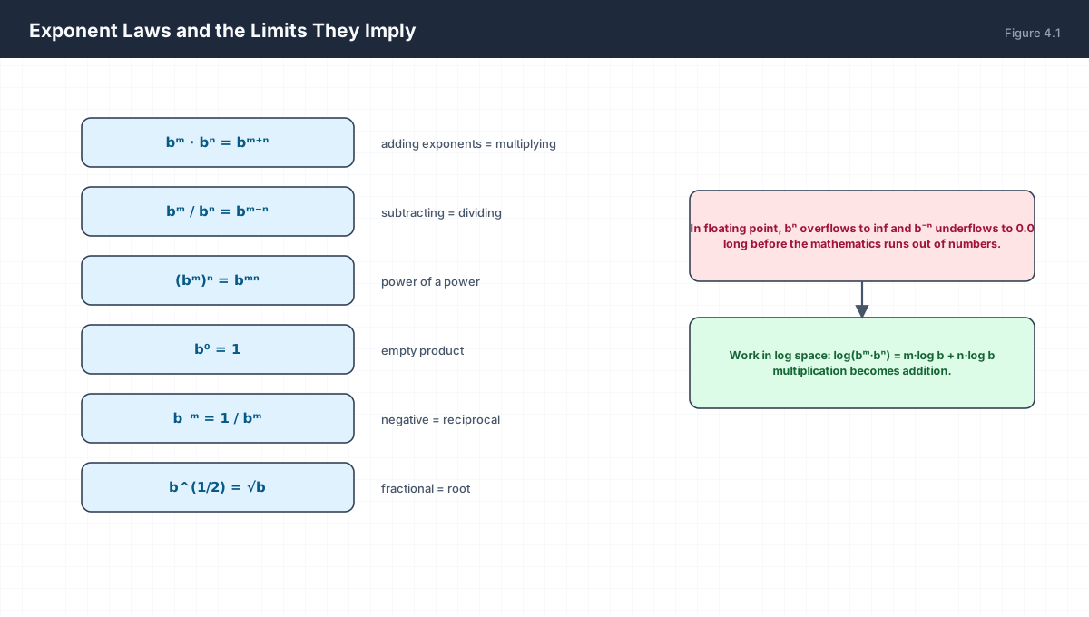
| Exponent Law | Logarithm Law | Why It Matters |
|---|---|---|
bᵐ·bⁿ = bᵐ⁺ⁿ |
log(xy) = log x + log y |
Joint log-probability of independent events is a sum |
bᵐ/bⁿ = bᵐ⁻ⁿ |
log(x/y) = log x − log y |
Log-odds are a difference of log-probabilities |
(bᵐ)ⁿ = bᵐⁿ |
log(xⁿ) = n·log x |
Perplexity = exp(mean NLL) |
b⁰ = 1 |
log 1 = 0 |
A perfectly predicted event costs nothing |
b⁻ᵐ = 1/bᵐ |
log(1/x) = −log x |
Negative log-likelihood is a positive cost |
The first row is the load-bearing one. A sequence of n independent token probabilities multiplies to the sequence probability; taking logs turns that product into a sum, which is numerically stable, differentiable, and trivially parallelisable across a batch. This single identity is why language models train in log space.
4. Log Scale: When a Straight Line Means “Constant Ratio”
On a linear axis, 2ˣ is invisible near zero and off the chart by x = 10. On a log axis it becomes a straight line, because log₂(2ˣ) = x.
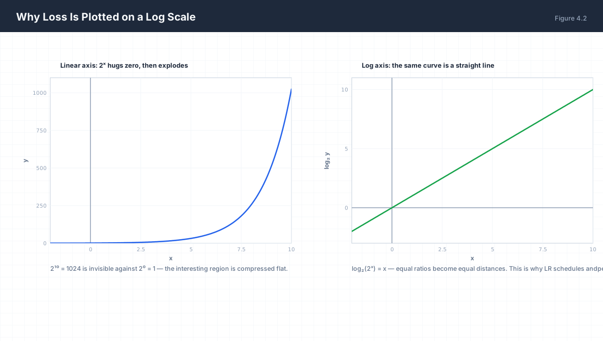
This is the correct axis whenever the quantity is a ratio rather than a magnitude:
- Loss curves. A training loss falling from
2.0to0.2is a 10× improvement whether it happens at epoch 1 or epoch 50. On a linear axis the early progress dominates and the interesting tail is flat. - Perplexity. Defined as
exp(NLL), so it is inherently multiplicative. - Learning rate schedules. Cosine versus exponential decay differ by orders of magnitude at the tail; only a log axis shows it.
- Parameter magnitudes. Weight distributions spanning
10⁻⁶to10⁰are unreadable linearly.
The practical reading rule: on a log-y plot, a straight line means exponential change; a concave curve that flattens means the change is slowing in ratio terms, which is what a well-behaved training run looks like.
5. Softmax: From Logits to a Distribution
A classifier produces raw scores called logits. They can be any real number, negative or positive, unbounded. We need a probability vector: positive entries summing to one. Two requirements, two steps.
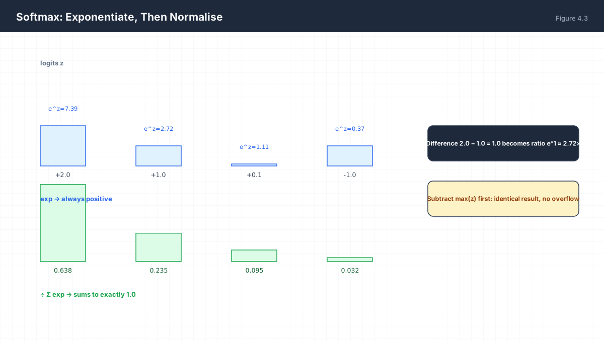
softmax(z)ᵢ = e^zᵢ / Σⱼ e^zⱼ

Why exp and not something else?
  exp is strictly positive  →  every class gets non-zero probability
  exp is strictly increasing →  order of logits is preserved
  exp turns differences into ratios:
        e^(a−b) = e^a / e^b
  so a logit gap of 1.0 always means the same odds ratio, regardless of scale.
import numpy as np

def softmax(z):
    z = np.asarray(z, dtype=float)
    z = z - z.max()            # shift: identical result, no overflow
    e = np.exp(z)
    return e / e.sum()

z = np.array([2.0, 1.0, 0.1, -1.0])
p = softmax(z)
print("probs:", np.round(p, 4))     # [0.6381 0.2347 0.0954 0.0318]
print("sum  :", p.sum())            # exactly 1.0
print("gap 2 vs 1 -> ratio", np.round(p[0] / p[1], 4), "= e^1 =", np.round(np.e, 4))
The ratio property is the reason softmax is used rather than simple normalisation. Dividing by the sum would also produce a distribution, but the numbers would depend on the arbitrary origin of the logits. With softmax, only differences matter: adding a constant to every logit leaves the output unchanged, which is why the max-subtraction trick is mathematically free.
6. Information Content and Cross-Entropy
Information theory asks: how surprising is an event, and how many bits does it cost to encode? The answer for an event of probability p is −log₂ p.
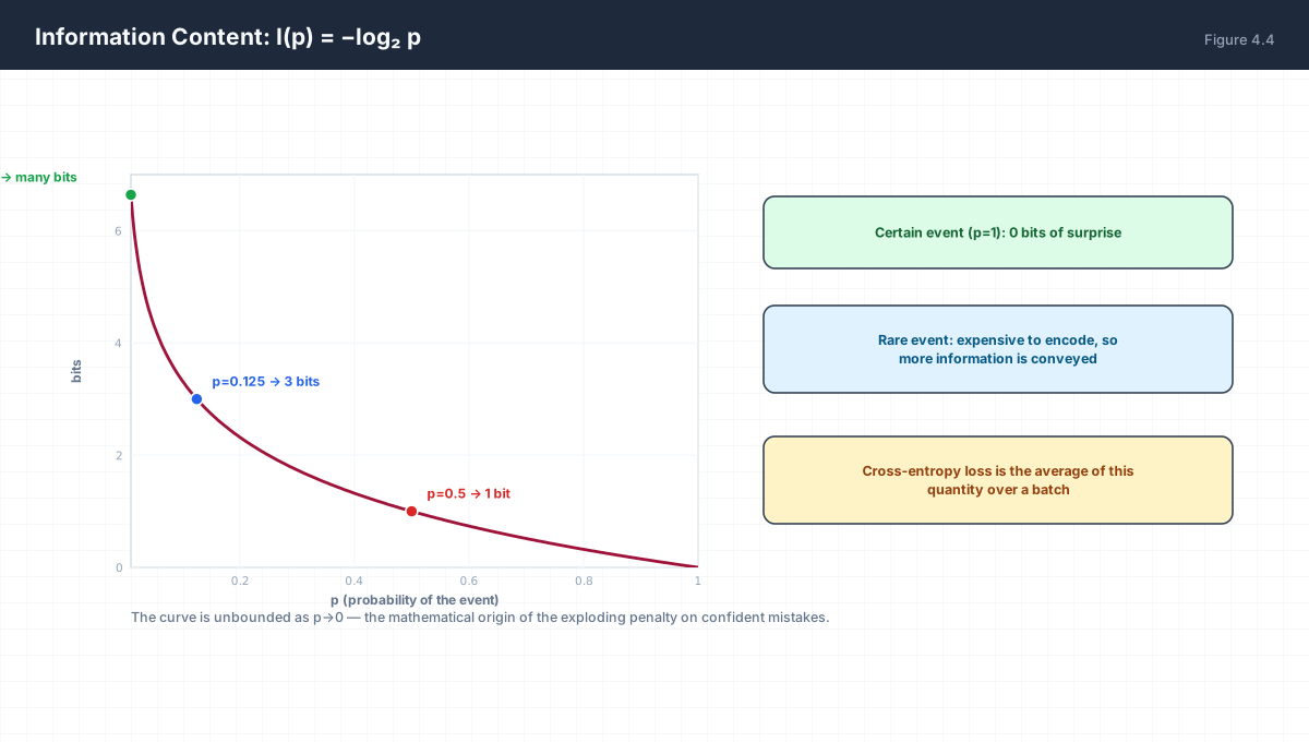
| Quantity | Formula | Interpretation |
|---|---|---|
| Information | I(p) = −log p |
Surprise of one outcome |
| Entropy | H(p) = −Σ pᵢ log pᵢ |
Average surprise of a distribution |
| Cross-entropy | H(p,q) = −Σ pᵢ log qᵢ |
Cost of encoding true distribution p with model q |
| Perplexity | exp(H(p,q)) |
Effective number of equally-likely choices |
For one-hot labels — the standard classification case — cross-entropy collapses to −log q_y where y is the true class. That is the negative log-probability the model assigned to the correct answer. The unbounded behaviour as q_y → 0 is precisely why a confidently wrong prediction is punished so heavily.
import numpy as np

def cross_entropy_one_hot(q, y):
    q = np.asarray(q, dtype=float)
    return -np.log(q[y])

q = np.array([0.7, 0.2, 0.1])
print("correct, confident  :", round(cross_entropy_one_hot(q, 0), 4))   # 0.3567
print("correct, unsure     :", round(cross_entropy_one_hot(q, 2), 4))   # 2.3026
print("confidently wrong   :", round(cross_entropy_one_hot(np.array([0.001, 0.001, 0.998]), 2), 4))

print("perplexity from NLL :", round(np.exp(0.6931), 4))   # ~2.0 classes
7. Where Floating Point Breaks
exp grows fast enough to leave the representable range of a 64-bit float on inputs that arise routinely in a transformer.
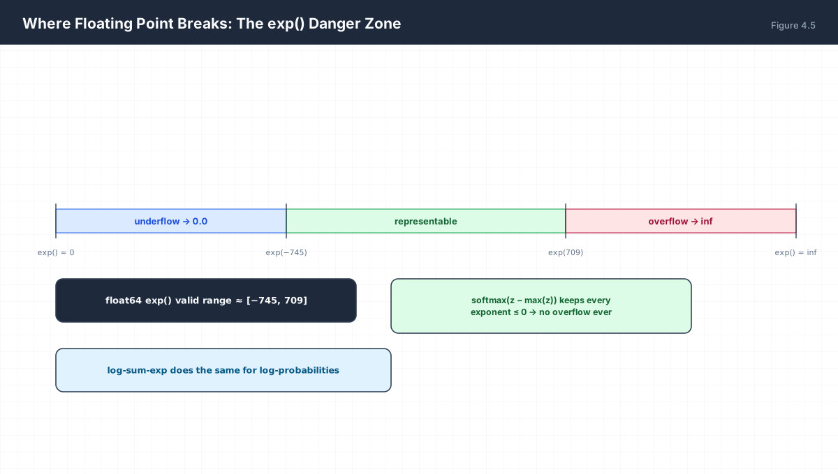
exp, and the two standard escapes: max-subtraction and log-sum-exp.import numpy as np
# Naive softmax on large logits
z = np.array([1000.0, 1001.0, 1002.0])
with np.errstate(over="ignore"):
naive = np.exp(z) / np.exp(z).sum()
print("naive:", naive) # [nan nan nan] -- inf/inf
# Max-subtracted version: identical maths, stable
zs = z - z.max()
safe = np.exp(zs) / np.exp(zs).sum()
print("safe :", np.round(safe, 6)) # [0.09 0.2447 0.6652]
# log-sum-exp: compute log(Σ exp(x)) without exponentiating the max
def logsumexp(x):
m = np.max(x)
return m + np.log(np.exp(x - m).sum())
print("logsumexp:", round(logsumexp(np.array([1000.0, 1001.0, 1002.0])), 4))
# 1002.4076 -- finite, although exp(1002) is inf
Both tricks rest on the same identity: subtracting a constant from every exponent is equivalent to dividing the whole expression by eᶜ, and a common factor cancels in a ratio. Choosing c = max(z) guarantees every exponent is ≤ 0, so no exp can overflow.
8. Worked Examples
8.1 Collapsing a product to a sum
A model assigns probabilities 0.5, 0.25, 0.125 to three independent tokens. Compute the sequence probability and its negative log.
P = 0.5 × 0.25 × 0.125 = 0.015625
−ln P = −(ln 0.5 + ln 0.25 + ln 0.125) = 0.693 + 1.386 + 2.079 = 4.159
8.2 Converting bits to nats
An entropy of 3 bits per token is how many nats?
1 bit  = ln 2 ≈ 0.6931 nats
3 bits = 3 × 0.6931 = 2.079 nats
8.3 Reading a perplexity
A language model reports perplexity 20. What average negative log-likelihood does that correspond to?
PPL = exp(NLL)  →  NLL = ln(20) = 2.996 nats/token
In bits: 2.996 / 0.6931 ≈ 4.32 bits per token
Interpretation: the model is as uncertain as choosing uniformly among 20 options.
8.4 Why the max-shift is exact
Show that softmax(z) = softmax(z − c) for any constant c.
e^(zᵢ−c) / Σⱼ e^(zⱼ−c)
  = (e^zᵢ · e^(−c)) / (Σⱼ e^zⱼ · e^(−c))
  = e^zᵢ / Σⱼ e^zⱼ        the factor e^(−c) cancels
8.5 Information content of a rare event
A token with probability 10⁻⁵ carries how many bits?
−log₂(10⁻⁵) = 5 × log₂ 10 = 5 × 3.3219 ≈ 16.6 bits
9. Verify It in Python
import numpy as np

# --- 1. Log laws hold ----------------------------------------------
x, y = 8.0, 32.0
assert np.isclose(np.log(x * y), np.log(x) + np.log(y))
assert np.isclose(np.log(x / y), np.log(x) - np.log(y))
assert np.isclose(np.log(x ** 3), 3 * np.log(x))
print("log laws verified")

# --- 2. Base conversion --------------------------------------------
bits = -np.log2(1e-3)
nats = -np.log(1e-3)
assert np.isclose(bits, nats / np.log(2))
print(f"p=1e-3 -> {bits:.4f} bits = {nats:.4f} nats")

# --- 3. Softmax invariants -----------------------------------------
def softmax(z):
    z = np.asarray(z, float)
    z = z - z.max()
    e = np.exp(z)
    return e / e.sum()

z = np.array([2.0, 1.0, 0.1, -1.0])
p = softmax(z)
assert np.isclose(p.sum(), 1.0)
assert np.all(p > 0)
assert np.isclose(p[0] / p[1], np.e)          # gap of 1.0 -> odds e
assert np.allclose(p, softmax(z + 100.0))     # shift invariance
print("softmax:", np.round(p, 4), "sum =", p.sum())

# --- 4. Naive softmax fails, shifted version survives --------------
big = np.array([1000.0, 1001.0, 1002.0])
with np.errstate(over="ignore", invalid="ignore"):
    naive = np.exp(big) / np.exp(big).sum()
assert not np.all(np.isfinite(naive))         # nan
print("naive on big logits:", naive)
print("safe  on big logits:", np.round(softmax(big), 6))

# --- 5. log-sum-exp stays finite -----------------------------------
def logsumexp(a):
    m = np.max(a)
    return m + np.log(np.exp(a - m).sum())

val = logsumexp(big)
assert np.isfinite(val)
assert np.isclose(val, np.log(np.exp(big - 1002.0).sum()) + 1002.0)
print("logsumexp:", round(val, 4))

# --- 6. Cross-entropy and perplexity -------------------------------
q = np.array([0.7, 0.2, 0.1])
nll = -np.log(q[0])
print("NLL for true class 0:", round(nll, 4))
print("perplexity of uniform-3:", round(np.exp(-np.log(1/3)), 4))   # 3.0
print("all assertions passed")
10. Practice Questions
- Simplify
(2³)² · 2⁻⁴and verify the result with logarithms. - Express
log₂(64),ln(e³), andlog₁₀(0.01)without a calculator. - Why must the base of
expin softmax match the base used in the cross-entropy that follows it? - Prove that softmax is invariant to adding a constant to all logits.
- A model outputs logits
[10, 9]. Compute the probability of the first class; then recompute after adding 1000 to both. - Explain why
−log pis unbounded asp → 0, and what that implies for label smoothing. - Convert a perplexity of 8 into bits per token.
- State the smallest and largest
xfor whichnp.exp(x)is finite in float64. - Why does
log-sum-expavoid overflow even when every input exceeds 700? - A loss curve is a straight line on a log-y plot. Describe the underlying decay.
11. Official References & Further Reading
Continue the Course
- Course Index: AI Mathematics Masterclass — All 48 Chapters
- Previous Chapter: Chapter 3: Functions, Graphs & Transformations
- Next Chapter: Chapter 5: Summation Notation, Sequences & Series
- Related Series: PyTorch Engineering Masterclass — All 16 Modules